A Procedural Model for Interactive Animation of Breaking Ocean Waves Stefan Jeschke
Hermann Birkholz
Heidrun Schmann
University of Rostock, CS Dept., Institute for Computer Graphics, Albert-Einstein-Str. 21, 18051, Rostock, Germany
University of Rostock, CS Dept., Institute for Computer Graphics, Albert-Einstein-Str. 21, 18051, Rostock, Germany
University of Rostock, CS Dept., Institute for Computer Graphics, Albert-Einstein-Str. 21, 18051, Rostock, Germany
Stefan.Jeschke@informatik. uni-rostock.de
[email protected]
[email protected]
ABSTRACT This paper presents a procedural model for breaking ocean waves that is intended to be used for interactive visualization. The movement as well as the appearance of the waves is modelled by a set of functions in dependence of time and space. This continuous surface description allowes it to calculate all properties of every point (including foam) on the ocean surface at every time without any information from previous time steps. By using an adaptive sampling sheme for rendering, the frame rate of the animation only depends on the screen resolution rather than on the model size. The model is quite simple, easy to implement, fast to compute and provides a visual appealing interactive animation of infinite large ocean coast scenes. On the other hand it provides only limited flexibility due to its procedural character. For achieving more realistic scene appearance, it may also easily be combined with models for deep-water waves presented in the past.
Keywords interactive, rendering, procedural modelling, ocean modelling, animation, water waves
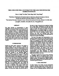
1. INTRODUCTION The modelling and visualization of ocean scenes has been a challenge in computer graphics for a long time. This paper focusses on the special case of interactive (this means at least 5 frames per second) visualization of plunged breaking waves in infinite large ocean coast scenes. The goal is a simple to implement and fast to compute model for producing high output frame rates and reasonable image quality. Figure 1 shows an output image generated by using this model (in combination with wave ripples modelled with sinusoids). The basic principle implemented here for achieving these goals is a procedural model. This means, every point in the ocean scene is described by some simple formulas in dependence of time and space. The ocean animation is then restricted to a continuously Permission to make digital or hard copies of all or part of this work for personal or classroom use is granted without fee provided that copies are not made or distributed for profit or commercial advantage and that copies bear this notice and the full citation on the first page. To copy otherwise, or republish, to post on servers or to redistribute to lists, requires prior specific permission and/or a fee. WSCG POSTERS Proceedings WSCG’2003, February 3-7, 2003, Plzen, Czech Republic. Copyright UNION Agency – Science Press
Figure 1: Output image generated with the presented method and wave ripples (sinusoids). changing parametrization for the formulas. The advantages of a procedural approach are a continuous surface description in time and space so that the location and appearance of every point in the scene can always be calculated without using information from previous time steps. Note especially, that even foam generated by the breaking waves will also be computed without recomputation of values obtained in previous time steps (in contrast to particle systems). Furthermore, the model can easily be used in combination with wave models for deep-water waves and fine rippling waves to enhance the realism.
On the other hand, a procedural model has the limitation that the oceans appearance and behaviour is completely defined by the author (such as wave refraction on the cost). This implies a reparametrization of the model for changing environment conditions (for instance a different coastline). Because a reparametrization done always by hand is not desireable, future work should focus on this to provide a more flexible use of the model. For displaying the ocean surface, a polygon mesh is generated by using the image space sensitive sampling method presented by Hinsinger [Hin02]. By using this rendering method, the output frame rate only depends on the screen area covered by the ocean field (i.e. the number of sampling points). Efficient use of current graphics hardware is provided due to the use of polygon strips. Since the model is easy to implement and provides fast output image computation, its main applications are virtual environments and computer games (also because simple collision detection is possible) as well as multimedia applications (think about a fly over an infinite large ocean surf scene).
2. RELATED WORK Early approaches in the field of ocean modelling and visualizing by Max [Max81], Fournier [Fou86], Peachey [Pea86] and Tso [Tso87] were able to produce fairly realistic results for relatively quiet ocean surfaces (also called "deep-water waves") but plunged breaking waves could not be modelled correctly due to the sinusoidal assumption in the parametric surface and/or the use of a high field wave representation. A good introduction and overview of that work is given in the SIGGRAPH 2001 course notes [Tes01]. More recent work by Jensen [Jen01] uses different wave modelling approaches for different levels of detail for interactive deep-water animation. There was also presented a texture-based method for rendering foam (that is also used in this paper) and show clever use of current graphics hardware to achive more realism. Extensive use of programmable graphics hardware was also done by Schneider [Sch01]. Here it was used for displacement, transformation and lighting calculations of a height field water surface for realizing effects such as refraction, reflection and the Fresnel term. Smith [Smi02] used in his diploma thesis surface markers to track a wave surface for interactive animating curling and breaking (including plunged) waves arriving at a coast. The most closely related work to this paper was made by Hinsinger [Hin02]. Here, procedural waves are
used to model an infinite large deep-water surface. The surface is rendered by using an adaptive sampling method that completely decouples the output frame rate from the size of the ocean scene. This paper can be seen as an extension of that work for handling breaking waves and the resulting foam.
3. A PROCEDURAL WAVE FIELD For further descriptions the basic coordinate setup illustrated in figure 2 is used (z is pointing up). The intial assumption for the procedural model is that all waves are straightly running towards the beach. For realistic wave behaviour, the phenomenon of wave refraction is modelled. This includes a slowing down of the wave when arriving the beach as well as a beach alignment.
Figure 2: Setup for the procedural wave field At first, a parameter s running from 0 to 1 over the wave’s life time is defined by using the time of birth (tstart) and dead (tend) of the wave and the current time (tcurrent):
t −t s = current start t end − t start
r
Here r defines the amount of deceleration and alignment to the coastline over time. The desired y position (ycurrent) for the current time (tcurrent) is then obtained by using: ycurrent = (1-s)ystart (x) + s yend(x) ystart is here a constant function so that the waves start as straight lines, whereas other functions are of couse also possible. yend defines the coastline. It can be defined by using a function in dependence of x (for instance a superimposition of sinus functions) or by using cubic interpolation of sampling points. Slightly varying values for r and/or yend let every wave run a bit on its own which gives a more natural look. The second phenomenon modelled here is the wave breaking. Normally, a wave begins to break at several points and then successively breaks over its whole width. This is modelled here by using a simple function tbreak(x) that defines the time the wave breakes for every point in x direction (for instance also a superimposition of sinus functions). Again, using slighly varying values for the function parameters lets every wave look unique.
3.1 Modelling Foam The foam modelled here is produced by breaking waves when the water from the top crashes into the
water at the bottom. Afterwards, foam slowly disappears when the milliards of small bubbles disappear. Because the breaking time for every wave is always known from its function tbreak(x), it is possible to compute the amount of foam for every point at the ocean surface at every time. For estimating the foam amount at a given point (x,y) at the current time tcurrent, all waves recently passed y are considered. For every wave, the exact time twave when it passed y is estimated by reorganizing the two functions above to tcurrent: r twave = tstart + (tend-tstart)
y-ystart yend-ystart
If the wave produced foam at that moment (this can simply be tested by using the function for breaking) the foam amount is faded over time by using a function that uses as input the time difference between twave and tcurrent (for the simplest case, this is a linear function). Finally, the highest foam value from all considered waves is taken as the actual foam value for that point.
4. PROCEDURAL WAVE SHAPES For procedural modelling the following basic "life cycle" of a breaking wave is considered (refer to figure 3). When a wave is born, it comes up from ocean level and has a round shape (a). When it breaks, the front part dents inside and the top part falls down thus forming a tube (b). Afterwards, the wave collapses until it is completely flat again (c).
(a)
(b)
(c)
Figure 3: Phases of the life cycle of a breaking wave. The basic idea for procedural modelling the wave shapes is to use a combination of four functions: cosines function, exponential function, rotation and scaling. Figure 4 illustrates this basic principle.
(a)
(b)
(c)
Figure 4: Example for a procedural wave shape. (a): combination of cosine, exponential and scaling function; (b): rotation; (c): scaling. For wave animation, the function parametrization is blended over time. The formulas and parametrization presented here are obtained by experiment using only visual control, whereas physically-based wave shape modelling would of course also be possible here. The functions map an input space parameter s (0≤s