Behavior Research Methods, Instruments, & Computers 2000.32 (1), 191-196
P-SPACE: A program for simulating spatial behavior in small groups VICENy QUERA, ANTONISOLANAS, LLUISSALAFRANCA, FRANCESC S. BELTRAN, and SALVADOR HERRANDO University ofBarcelona, Barcelona, Spain P-SPACE is a computer program that simulates spatial behavior in a small group of individuals. The program describes how interpersonal distances change through time as a result of changes in microlevel features, such as the minimization of local dissatisfaction. Agents are located in a two-dimensional lattice and can move some discrete space units at each discrete time unit within their neighborhood. A nonsyrnmetrical matrix of ideal distances between agents must be specified. Agents move in order to minimize their dissatisfaction, defined as a function of the discrepancy between possible future distances and ideal distances between agents. At each iteration, agents will move to those cells in their neighborhoods for which the function is minimized. Depending on the specific values in the ideal-distance matrix, different kinds of social dynamics can be simulated.
Personal space-that is, how close someone will approach other people and how close he or she will allow other people to approach him or her-was mainly studied by Hall (1966), who introduced the term proxemics. Accordingly, personal space is usually defined as an area surrounding individuals during their interactions with others that expands or contracts, depending on current conditions (Little, 1965). When an individual intrudes on another's personal space, the action causes the second person discomfort. Empirical research has pointed out some factors influencing the size of this area, such as age, gender, and personality, but the most relevant factors are cultural differences (Hayduk, 1983). Because personal space is related to crowding and territoriality, it is also a main field of interest for environmental psychologists (Cassidy, 1997). However, studies of personal space in social psychology have usually been descriptive, rather than having a mathematical orientation. Recently, it has been proposed that cellular automata (CA) offer a promising avenue for understanding social dynamics (Hegselmann, 1996; Hegselmann & Flache, 1998). From this point of view, social and psychosocial macro effects could be explained from micro level behavior. In other words, we can simulate many kinds of complex social behavior only by establishing relations between individuals or by specifying behavioral rules for them. The Preparation of this paper was supported by Direcci6n General de Ensefianza Superior (Spanish government) Grant PB96-1489 and Cornissionat per a Universitats i Recerca (Catalan autonomous government) Grant I997SCR-00344 to the Grup de Tecnologia Informatica en Ciencies del Comportament. We thank Thierry Cezard, Vicenta Sierra, Jose Manuel Juarez, Montse Girabent, Nuria Julia, Meritxell Mifiano, and Alba Mas for their help and suggestions, Correspondence concerning this article should be sent to V Quera, Departament de Metodologia de les Ciencies del Comportament, Facultat de Psicologia. Universitat de Barcelona, Passeig Vall dHebron 171,08035 Barcelona, Spain (e-mail:
[email protected]).
main elements and concepts in CA theory (Gaylord & Nishidate, 1996; Wolfram, 1994) are that (l) There is a lattice or array in one, two, or three dimensions (i.e., a CA can be a string, a grid, or a solid made up of elementary cells); (2) each cell can be in a single discrete state (usually on/off) at each discrete time; (3) a set of transition rules is defined, specifying the state of every cell at time t as a function of the states ofthe cells in its neighborhood at times t - 1, t - 2, '" , although usually only time t - 1 is considered (i.e., a CA has spatial and temporal locality); and (4) transition rules are usually applied homogeneously and simultaneously to every cell in the lattice at every time t but can also be applied heterogeneously and randomly. Different types of two-dimensional neighborhoods have been used. For a cell in the lattice, the von Neumann neighborhood is defined by its surrounding cells' being located to the north, south, east, and west. The Moore neighborhood includes cells in diagonal directions as well. Sakoda (1971) developed a model in which individuals, or agents, of two different groups live in a lattice. Attitudes between agents can be positive, negative, or neutral and are represented by integer values, which are called valences. Agents make the decision to move to an empty cell in their own Moore neighborhoods at every time unit or iteration of the process. The rule being used to decide their new positions in the grid consists of maximizing the weighted sum ofvalences for each agent. Schelling (1969) proposed a model in which agents live in cells on a line and individuals move to the left or the right in accordance with certain rules. This kind of model is referred to as a migration model in the literature, because agents move around the grid or the line positions. Unlike migration models, steady site models do not allow agents to move around them. These models are interesting for social researchers, because they make it possible to explain macro behaviors (groups or societies) from microlevel behavior. Migration models were implemented by Goldstein in his
191
Copyright 2000 Psychonomic Society, Inc.
192
QUERA, SOLANAS, SALAFRANCA, BELTRAN, AND HERRANDO
Party Planner program (Dewdney, 1987) and have been used to simulate artificial societies (Epstein & Axtell, 1996). In this paper, we present a migration model of social dynamics in which agents have attitudes towardeach other. Attitudes, or valences, are defined as euclidean distances measured in a lattice, and agents make the choice to move to those cells in their neighborhoods at which a dissatisfaction function is minimized (Dewdney, 1987). The main purpose of our model and of the P-SPACEprogram based on it is to help social psychologists investigate emergent structures in small groups.
MODEL DESCRIPTION
dij(t)=
[x j(t)-Xj
(t) ]2+[Yj(t)- y/t)f·
When objects are included, real distances between agents are computed as virtual trajectories around the interposed objects. At time t, agent i's ideal distance from agentj is Dj/t), and agentj's ideal distance from agent i is Djj(t). Ideal distances are not necessarily symmetrical and may be constant or vary as a function of time, proximity, or both. Certain ideal distances can be void-that is, agent i can be neutral with regard to agent). At time t, agent i's real dissatisfaction is computed as
L jE7 j
wij(t)·ldij(t)-Dij(t)1
U;(t) = - - - - - - - - , O~Uj(t)~1. m L Wij(t) The model includes agents, objects, and doors. Agent JET, is a general term that designates individuals, organisms, or robots that have the capacity to move in a universe, In that formula, T, is the set of agents for which agent i called a room, which may have doors. Objects are rectan- has nonneutral ideal distances; m is the longest possible gular restricted areas that cannot be accessed by agents. distance in the room and is used in the formula for scalIf the room has doors, agents may exit and enter the room ing dissatisfactions between 0 and 1; Wi/t) weights the by them. discrepancy between real and ideal distances, using a Let us suppose that n agents are in the cells of a lattice gravity parameter gj (0 < gj :::::; 1), which may be differ(representing n individuals in a room) and that their spa- ent for each agent: tial behavior is governed by their respective degrees of dij(t) social dissatisfaction. For every agent, social dissatisfacwj/t)=gj-m-. tion is defined here as a function of the discrepancy between its real distance from other agents and the ideal dis- Weight w/t) decreases exponentially as a function of tance it wants to keep from them. Dissatisfaction equals real distance, its decreasing rate becoming greater as gj approaches O. Thus, the greater the gravity, the higher zero only when ideal and real distances are identical. The model states that an agent's behavior (its movement the weighting of the differences between real and ideal in the room) will take place in such a way that its dissat- distances on dissatisfactions. The smaller the gravity, the isfaction will be minimized-that is, so that, in its new lower the weighting. When gravity is near 1, the effect of position, the real distances from the other agents are as those differences on dissatisfaction does not depend on similar as possible to the respective ideal distances. There- the real distances. When gravity is near 0, real distances fore, agents will keep moving in the room until their dis- must be small for the differences between real and ideal satisfactions are null. Nevertheless, it may be that, owing distances to affect dissatisfaction. In the special case in to the ideal distances of other agents, the null level of dis- which gravity equals 1, dissatisfaction is computed as the satisfaction is unreachable. In this case, the group as a scaled average of absolute differences between real and ideal distances. system can reach either static or dynamic stability. The model has the following restrictions and assumpWhen objects and doors are present, ideal distances tions: (1) Agents move in a lattice, occupying a single cell from agent to object and from agent to door are defined at a time (time and space are measured in discrete units); as well, analogously to ideal distances between agents. In (2) a cell cannot be occupied by two or more agents si- that case, additional agent-by-object, and agent-by-door multaneously; (3) agents make the decision to move in- ideal distance matrices must be specified. For example, dependently from the other agents at the same moment if agent i's ideal distance from door k is 0, the agent will (parallelism assumption); (4) in each time unit, agents can tend to approach door k and to exit the room through it. only move within their neighborhoods (locality assumpAgents have individual features: (I) the initial oriention); and (5) as was described above, agents' decisions are tation or heading, subsequent headings being defined by a function of their ideal and real distances from the other the direction of its movement from time t to time t + I; agents, and this function is the same for all the agents (ho- (2) attention scope, centered at its current heading and mogeneityassumption). defining the area within the room to which the agent At time t, agent i is located at position [xj(t), Yj(t)] in "pays attention" at time t, so that only other agents, obthe room. The origin ofthe coordinates is arbitrarily fixed jects, and doors lying in that area are considered when in the upper left corner of the room. The real distance be- computing the agent's dissatisfaction at that time; (3) gravity; (4) initial place, either in or out of the room; tween agents i and j at time t is
SIMULATING SPATIAL BEHAVIOR
(5) initial position within the room, ifthe agent is initially in the room; (6) time-out expectancy (i.e., when an agent exits the room, its actual time out is sampled from an exponential distribution with that expectancy); (7) the tendency to exit the room if, by chance, the agent falls on a door threshold; and (8) the door used for reentering the room, which can be either the same door through which the agent exited the room or a randomly chosen door. A neighborhood surrounds each agent at time t. Different types of neighborhoods can be used-Moore's, von Neumann's, Moore-von Neumann's, or circular-and these can have different diameters (Gaylord & Nishidate, 1996). The diameter and type of neighborhood are the same for all the agents. Depending on the actual type of neighborhood, certain movements are favored; for example, in a von Neumann neighborhood, movements can only be in vertical and horizontal directions, whereas in a circular one, movements are isotropic. Moreover, the longer the diameter, the faster the movements can be. Agent i computes its ideal, or future, dissatisfactions for all possible positions within its neighborhood at time t + I, assuming the other agents will not move. Then, agent i decides to move to the position having the minimum ideal dissatisfaction, provided that that position is available (i.e., it lies within room boundaries and is not occupied by another agent). The order in which agents decide to move is randomized at each time unit. Of course, some agents may not move at all if their current positions already provide minimum dissatisfactions. Once agent i has moved to a certain position, its real dissatisfaction does not necessarily equal the ideal one that was predicted for that position, because the other agents also may have moved. The difference between ideal dissatisfaction (predicted at time t for time t + I) and the real dissatisfaction at time t + I is the agent's frustration at time t + I. Agents will keep moving so long as their dissatisfactions do not reach an overall minimum. Depending on the actual values in the ideal-distance matrix, a group of agents can reach either a steady state or a dynamic equilibrium. For example, the following agent-by-agent idealdistance matrix generates a steady state: 5 5 5
5
5 5
5 5
5 5 5
5
Agents will move from their initial positions to a point at which their mutual real distances equal the ideal distances in the matrix. The following matrix generates a perpetual persecution: 2 20 10 2
10
2 20 10
20 10 2
20
Agents cannot reach a point at which the real distances equal their ideal ones and keep moving and "chasing" each
193
other (Agent I chases Agent 2. Agent 2 chases Agent 3; and so on). The following types of ideal distances can be defined for each off-diagonal cell in the matrix: (1) neutral, if agentj's position does not affect agent i's dissatisfaction; (2) constant, if the ideal distance from agent i to agent) does not vary as the simulation progresses (the above matrices are examples of constant ideal distance for every pair of agents); (3) random, if the ideal distance from agent i to agent) is uniform and randomly distributed between two values; (4) sociable, if the ideal distance from agent i to agent) decreases with time after the simulation has started until a lower limit is reached; (5) unsociable, if the ideal distance from agent i to agent) increases with time after the simulation has started until an upper limit is reached; (6)fatigue, if the ideal distance from agent i to agent) increases as a function of their proximity (an initial ideal distance exists, but, if agent) happens to be nearer than a certain critical distance for longer than a certain critical time, the ideal distance increases for a certain period; once the time limit is reached, the ideal distance regains its initial value); and (7) deprivation, if the ideal distance from agent i to agent) decreases as a function of their proximity (an initial ideal distance exists, but, if agent) happens to be farther than a certain critical distance for longer than a certain critical time, the ideal distance decreases for a certain period; once the time limit is reached, the ideal distance regains its initial value). These types of ideal distance can be defined for agent-by-object and agent-by-door matrices as well. lt is possible to specify different types of ideal distances for each interaction or cell in the matrix. For example, the ideal distance between agents i and) may be constant, but the ideal distance between agents) and i may be sociable. When more than two agents are included and different types (and/or different parameter values) of ideal distances are specified, the exact trajectories and future positions of the agents in the room are usually difficult to predict. When variable ideal distances are specified, ideal-matrix values can change at each iteration. Moreover, if fatigue or deprivation ideal distances are specified, the outcome ofthe simulation tends to be rather complex, because ideal distances change as a consequence of the behavior of the other agents.
RUNNING P-SPACE The P-SPACE program simulates spatial behavior in a small group (up to 20 agents) in accordance with the minimum dissatisfaction model. Two versions of P-SPACE have been developed, one for DOS and one for Windows 95/98. Both versions read commands and parameter specifications from an ASCII file and graphically display the agents' positions, trajectories, real and ideal distances, and real dissatisfactions as a function oftime. Ifrequested, results are exported to a file, to be subsequently analyzed by SPSS, StatGraphics, or Excel. P-SPACE for Windows
194
QUERA, SOLANAS, SALAFRANCA, BELTRAN, AND HERRANDO
can also accept input from dialogue windows and can save parameters in command files. The program inputs are ( I) the number of simulations or the number of replications, using the following set of parameters; (2) the time per simulation; (3) the room size, width X length; (4) the number of agents; (5) the agents' individual features, including their initial coordinates within the room (which can be randomly assigned), initial headings, attention scopes, gravities, and so on; (6) the number of rectangular objects in the room, which can be zero; (7) the object coordinates; (8) the number of doors in the room, which can be zero; (9) the door coordinates; (10) the type of neighborhood and its diameter (3,5,7, ...); (11) the ideal-distances matrix; and (12) the output, which can be graphical, given in ASCII, or both. Users can also select an icon for representing the agents, decide whether their trajectories are to be shown, specify certain output variables to be plotted, and specify whether the program should pause or not between successive time units. For example, this command file requests 10 replications of a simulation involving four agents with default individual features:
tion. And F 2 20 I 50 100 would indicate a fatigue ideal distance, which is initially kept constant at 2 but linearly increases up to 50 during 100 time units whenever the two agents are closer than I (real distance) for longer than 20 consecutive time units. A sample screen of a simulation is shown in Figure I. The upper left rectangle shows three agents moving in an 80 X 70 room containing one object and two doors. Their dissatisfactions (labeled AgDss, for agent dissatisfaction) as a function oftime are shown below. That simulation was produced by the following commands: Nsimulations 10 Time 100 Room 80 70 Block 3 -1 360 lOin random exit Door north 40 Door west 30 Object 35 20 55 40 Gravity 0.5 all
Nsimulations 10
Neighborhood circular 5
Time 500
Rectangle dissatisfaction
Room 80 60
Square distance
Neighborhood Moore 5
Trajectory yes
Nagents 4
Output all SPSS
Output all SPSS
Ideal user
Ideal user
N
S 40
100 U
N
C2
C 10
C 20
U 1 40 100 N
C20
N
C2
C 10
S 40 I 100 U 2 20 100 N
C 10
C20
N
C2
C2
CIO
C20
N
Ideal distances are specified immediately after the "Ideal user" command. Since there are four agents and no objects or doors, this matrix is 4 X 4. In the matrix cells, letters are used for specifying types of ideal distance. In the above example, all off-diagonal cells contain a C, which stands for constant ideal distance. The numbers after the Cs indicate the distances. Diagonal cells contain N, or neutral ideal distance. For example, the ideal distance from Agent 1 to Agent 2 is C 2, whereas the ideal distance from Agent 2 to Agent 1 is C 20. This specific matrix will generate a circular persecution, with Agent 1 chasing Agent 2, Agent 2 chasing Agent 3, Agent 3 chasing Agent 4, and Agent 4 chasing Agent 1. More parameters are necessary in a cell in order to specify a variable ideal distance. For example, S 10 4 50 would indicate a sociable ideal distance, linearly decreasing from 10 to 4 in the first 50 time units of the simula-
I 40 100 N N N
S 40 I 100 N N N NNN
Command "Block" is used for defining the following: three agents with identical features-in this case, with random initial headings (-I); full attention scopes (360°); a time-out expectancy equal to 10 time units; initially in the room; a randomly chosen door for reentering the room; and a tendency to exit the room if agents fall, by chance, on a door threshold. Commands "Door" and "Object" define coordinates for doors and object. Commands "Rectangle" and "Square" specify the variables to be plotted in the lower left rectangle and the lower right square, respectively. Finally, the ideal-distance matrix has three rows (one per agent) and five columns (for Agents I, 2, and 3, Object I, and Doors 1 and 2, respectively). In the figure, the lower right 3 X 3 grid contains representations of ideal and real distances between agents as a function oftime (ideal and real distances from agents to object and doors are not shown). The horizontal and vertical axes in each square of the 3 X 3 grid represent time (from 0 to 100 in this example) and distance (from 0 to 106, which is the maximum distance in the room-i.e.,
SIMULATING SPATIAL BEHAVIOR its diagonal), respectively. For example, in the 3 X 3 grid, the square in the first row, second column, shows how the ideal distance from Agent I to Agent 2, or D l 2 (t), changed as time progressed. The square is labeled S (for sociable) because the model specified for that cell in the idealdistance matrix was S 40 I 100, which defines a straight line starting at ideal distance 40 at time 0 and decreasing linearly with slope (1-40)/1 00 until time 100-that is, the ideal distance from Agent 1 to Agent 2 will be progressively smaller. The real distance from Agent 1 to Agent 2 is shown (using a different color in a real screen) in the same square as a slightly curved line approaching the ideal-distance line closely. Squares labeled U (for unsociable) contain straight lines with positive slopes, depicting how ideal distances increase as a function oftime for those particular agent-to-agent interactions. Curved lines in those squares indicate how closely or not real distances follow ideal distances and, indirectly, which par-
or-,
195
ticular interaction is responsible for each agent's dissatisfaction as time progresses.
FINAL COMMENTS Previous research on personal space was distinctively biased toward qualitative and descriptive studies. Our approach is quantitative-that is, all implied concepts are defined operatively and can be quantified. Moreover, our model for spatial behavior is based on principles of CA theory, which may be helpful for explaining global and complex behavior based on simple, local rules. Thus, like computer models of artificial life (Adami, 1998; Langton, 1989), P-SPACE creates an emergent pattern of behavior that is usually difficult to predict from local rules. The model on which P-SPACE is based has yet to be validated. In order to validate it, empirical data about members' attitudes toward each other should first be gath-
~P--,S::.:.P..:..A""C=.E....:2=.-=2::.:..O:.:l'--.::.JS