JOURNAL OF IMAGING SCIENCE AND TECHNOLOGY® • Volume 48, Number 2, March/April 2004
A Psychophysical Experiment Evaluating the Color and Spatial Image Quality of Several Multispectral Image Capture Techniques Ellen A. Day, Roy S. Berns,▲☛ Lawrence A. Taplin, and Francisco H. Imai▲ Munsell Color Science Laboratory, Chester F. Carlson Center for Imaging Science, Rochester Institute of Technology, Rochester, New York, USA
Theoretically, there can be a compromise between color and spatial image quality for multispectral imaging: Increasing the number of channels increases spectral and colorimetric accuracy, that is, color quality increases; decreasing the number of channels reduces image noise and other spatial artifacts, that is, spatial image quality increases. Two paired comparison psychophysical experiments were performed to scale color and spatial image quality in order to better understand this compromise. Test targets, a watercolor painting, and several dioramas were imaged using three-, six-, and 31-channel image acquisition systems. One of the three-channel systems was a professional grade trichromatic digital camera; the other systems used the identical research grade sensor. For the six- and 31-channel images, both direct pseudoinverse based transformations and the use of principal component analysis were used to convert from digital to spectral data. The spectral data were used to render colorimetric images. Pseudoinverse transformations were used to convert the three-channel images to colorimetry. Twenty-seven observers judged, successively, color and spatial image quality of colorimetric images rendered for an LCD display compared with objects viewed in a light booth. The targets were evaluated under simulated daylight (6800K) and incandescent (2700K) illumination and the visual data were transformed to quality scales using Thurstone’s law of comparative judgments, Case V. The first experiment evaluated color image quality. Under simulated daylight, the subjects judged all of the images to have the same color accuracy, except the professional camera image that was significantly worse. Under incandescent illumination, all the images, including the professional camera, had equivalent performance. The second experiment evaluated spatial image quality. The results of this experiment were highly target dependent. A subsequent image registration experiment showed that the results of the spatial image quality experiment were affected by image registration to some degree. For both experiments, there was high observer uncertainty and poor data normality. Dual scaling and a graphical analysis of observer response data were used as alternate techniques to Thurstone’s Law. These techniques yielded similar results to the Thurstone-based quality scales. The uncertainty was caused by insufficient ambiguity between images. A simultaneous analysis of the color and spatial image quality results for the research grade sensor indicated that the most preferred image types were the 31-channel images. Thus, it is possible for multispectral images with many channels to achieve similar color and spatial image quality to systems with just a few channels. The theoretical compromise between color and spatial image quality as the number of channels increased was not observed under these experimental conditions. Journal of Imaging Science and Technology 48: 93–104 (2004)
Introduction Spectral image capture in the visible spectrum that is optimized for the precision and accuracy requirements of human visual observation has become an emerging topic of research, recently summarized by Hardeberg, et al.1 (see also Ref. 2). At the Munsell Color Science Laboratory, research in spectral image capture has been aimed towards archiving the optical properties of cultural heritage.3 It is our expectation that a spectral image archive provides many opportunities for new scholarship of this heritage and a range of practical applications including museum lighting design and color reproductions with vastly improved color quality, especially with respect to metamerism. Berns, et al. have summarized these opportunities.4 In general, the quality of a spectral imaging system is defined by the quality of the estimated spectra. Color targets Original manuscript received June 20, 2003 ▲ IS&T Member *
[email protected] Supplemental Material—Figures 1–5 and 10 can be found in color on the IS&T website (www.imaging.org) for a period of no less than two years from the date of publication. ©2004, IS&T—The Society for Imaging Science and Technology
are evaluated in which the spatially averaged estimated spectra using imaging are compared with spectra measured using small-aperture reflection spectrophotometers. Spectra are compared using colorimetric, spectral, and metameric criteria.5 As image data, there is an obvious requirement for viewing the spectral data in a rendered form such as display or print. When rendered, the many-channel data are mapped to three signals. That is, the high dimensional spectral data are projected onto the human visual system subspace (or an appropriate linear transformation). Similar to the conversion from spectral reflectance to tristimulus values using a reflection spectrophotometer, the accuracy can be quite high. Intuitively, as the number of channels increases, the spectral accuracy and in turn, the colorimetric accuracy is expected to increase. Unlike spectrophotometers, imaging systems are often subject to considerably greater noise. As noise is propagated through an imaging system,6 the rendered image may have poor spatial image quality and be quite objectionable. With the potential large number of channels and complex signal processing, spectral imaging seems susceptible to image noise.7 It is quite possible that the noise propagation during projection can result in rendered images with poor spatial image quality. In addition, as the number of channels increase, there is an
93
1
0.9
0.9
0.8
0.8
0.7
0.7
Normalized sensitivities
Normalized sensitivities
1
0.6 0.5 0.4
0.6 0.5 0.4
0.3
0.3
0.2
0.2
0.1
0.1
0 380 400
450
500
550
600
650
700
750
Wavelength (nm)
0 380 400
450
500
550
600
650
700
750
Wavelength (nm)
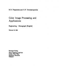
Figure 1. Normalized spectral sensitivities of the 31-channel capture system. Sensitivities include the sensor spectral sensitivities, infrared and ultraviolet blocking filter, and LCTF transmittances. Supplemental Material—Figure 1 can be found in color on the IS&T website (www.imaging.org) for a period of no less than two years from the date of publication.
Figure 2. Normalized spectral sensitivities of the six-channel capture system using six transmission filters optimized for both colorimetric and spectral measurements. Sensitivities include the sensor spectral sensitivities, infrared and ultraviolet blocking filter, and colored glass transmittances. Supplemental Material—Figure 2 can be found in color on the IS&T website (www.imaging.org) for a period of no less than two years from the date of publication.
increased probability of registration type errors. These potential rendering limitations can lead to visual artifacts including graininess, blurring, color fringing, contouring, and blocking. Thus, there is a potential compromise between color and spatial image quality. Intuitively, we recognized that the increase in information content that a spectral image affords does not offset a reduction in color and spatial image quality. Assuredly, evaluating cultural heritage will always be dominated by visual analyses. Accordingly, a visual experiment was performed in which observers scaled the quality of LCD rendered images from several multispectral image capture techniques in comparison to objects and test targets situated in a typical light booth. Different numbers of channels and different signal processing were considered. The results would provide benchmarks, observer thresholds, and a better understanding of image noise requirements in spectral imaging. The color accuracy experiments were summarized by Day, et al.8 The current publication describes the results of both visual tasks. Greater details can be found in Ref. 9.
channels yielded near-colorimetric spectral sensitivities. By placing a Wratten No. 38 light blue gelatin filter in front of the lens, a second triplet of channels was achieved. These spectral sensitivities are plotted in Fig. 3. (The choice of filter was based on previous research using a different sensor; clearly, there is an opportunity for greater differences in spectral sensitivity by using a different filter, a current research topic.) A professional quality RGB camera, a Nikon D1, was used in these experiments, as well. This camera incorporates a color filter array. The spectral sensitivities were unknown but believed to be typical of this technology. In total, there was one 31-channel system, two six-channel systems, and 2 three-channel systems, i.e., the Nikon and the Quantix with the three near-colorimetric filters. The 31- and six-channel systems were used to estimate spectral reflectance factor. The three-channel systems were used to estimate colorimetric coordinates. All imaging was performed in the Spectral Color Imaging Laboratory at the Center for Imaging Science at RIT. This laboratory is painted black to reduce unwanted flare and reflections. An easel was positioned against one wall and was used to hold all targets upright and perpendicular to the floor. Directly across from the easel was the camera (either the Nikon or Quantix) on an Industria Fototechnica Firenze Minisalon 190 monopod with a Bogen Manfrotto 3029 head. The ElinChrom ScanLite Digital 1000 studio lamps were set up facing the easel so that the the targets were illuminated at approximately 45° on either side. Between the camera and the rest of the set-up was a baffle of black paper, placed to minimize optical flare. For each channel, the exposure time was adjusted so that a pressed polytetrafluoroethylene (PTFE) tablet had average digital counts of 3800. In addition to the targets, images were captured of a gray card (for digital flat fielding) and with the shutter closed (to compensate for fixed-pattern noise). Each acquisition system required calibration in order to convert between digital counts and either spectral reflectance factor or colorimetric coordinates. A review of various techniques is described in Ref. 9. The GretagMacbeth
Image-Acquisition Systems A Roper Scientific Photometrics Quantix monochrome camera was coupled, at first, with a Cambridge Research and Instrumentation, Inc. liquid-crystal tunable filter (LCTF). The Quantix camera uses a Kodak KAF-6303E 2,048 × 3,072 sensor, a 12-bit analog-to-digital converter, and is thermoelectrically cooled. The spectral sensitivities and noise characteristics of this specific camera have been previously characterized.9,10 The LCTF was operated in its “low contrast” mode resulting in bandwidths ranging between 10 and 50 nm over the 400 to 700 nm wavelength range. The normalized spectral sensitivities of the 31 channels are plotted in Fig. 1. The Quantix was also coupled with a six position filter wheel. Six filters were fabricated such that the camera was effective for both spectral and colorimetric image acquisition.11, 12 The spectral sensitivities of these six channels are plotted in Fig. 2. Three of these six
94 Journal of Imaging Science and Technology®
Day, et al.
1 0.9
Normalized sensitivities
0.8 0.7
Baby
CC
CCDC
Fruit
Nature
Paint
0.6 0.5 0.4 0.3
Figure 4. Targets used in the visual experiments. Supplemental Material—Figure 4 can be found in color on the IS&T website (www.imaging.org) for a period of no less than two years from the date of publication.
0.2 0.1 0 380 400
450
500
550
600
650
700
750
Wavelength (nm)
Figure 3. Normalized spectral sensitivities of the six-channel capture system using three transmission filters optimized for colorimetric measurements and a Wratten 38 gelatin filter. Sensitivities include the sensor spectral sensitivities, infrared and ultraviolet blocking filter, and colored glass transmittances, and Wratten transmittance. Supplemental Material—Figure 3 can be found in color on the IS&T website (www.imaging.org) for a period of no less than two years from the date of publication.
ColorChecker DC was used as the calibration target in this research. A GretagMacbeth SpectroEye was used to measure the spectral reflectance factor of each patch. Colorimetric coordinates were calculated for the 1931 CIE standard observer and spectral power distributions used in the visual experiment based on spectral radiance measurements using a PhotoResearch PR-650. Detailed descriptions of the calibration transformations can be found in Ref. 13. In this research two different methods were used for each six-band system. Table I summarizes the various transformations used in this research and their abbreviations. For the 31-channel system, a pseudoinverse transformation was used, shown in its most basic form in Eq. (1). M(m,m) = R(λ,p*n)(D(m,p*n))T[(D(m,p*n))(D(m,p*n))T]–1
(1)
where M is the (31 × 31) transformation matrix, R is the matrix of measured spectral reflectances of the ColorChecker DC, and D is the matrix of the patch digital counts following spatial and fixed-pattern corrections. All the spatial and fixed-pattern corrections were unique for each channel, either for the LCTF or the six absorption filters. These corrections are critical for the LCTF; its transmittance varies significantly across the active area and as a function of wavelength. The subscript m represents the number of channels, in this case, 31 channels. The number of pixels per patch and the number of patches are represented by p and n, respectively. T denotes matrix transpose and –1 denotes matrix inversion. Typically, pseudoinverse transformations lead to poor results. In our case, each pixel was a separate datum. Several hundred thousand data points were used to estimate M. Under these conditions, the pseudo-inverse transformation produces acceptable results. This method is incorporating noise characteristics of the imaging system. Thus, this estimation technique is
similar to those that directly incorporate a noise model such as Wiener estimation.14 The MATLAB function pinv was used to implement the mathematics, which calculates the Moore–Penrose pseudoinverse of a matrix. The pseudoinverse transformation was also used to create (31 × 6) transformation matrices that converted digital data to spectral reflectance for the two six-channel systems. Much of our past research has used principal component analysis as an intermediate step between image acquisition and spectral reflectance estimation. 15 First, a set of eigenvectors was derived from the spectral reflectances of the calibration target. Based on preliminary analyses, six eigenvectors were used. The second part of the process included the pseudoinverse calculation to compute a transformation matrix: M(q,m) = (E(m,q))T[(E(m,q))(E(m,q))T]–1R(λ,p*n)(D(m,p*n))T [(D(m,p*n))(D(m,p*n))T]–1
(2)
where E is the matrix of eigenvectors and the subscript q is the number of eigenvectors (six, in this case). Thus, the pseudoinverse was used to relate camera signals with principal components, i.e., the eigenvector scalars. For the three-channel Quantix system, the pseudoinverse transformation technique was used to convert digital data to tristimulus values. For the Nikon system, “gamma” correction was first used to linearize the image data with respect to luminance factor. Two-degree polynomials were optimized using the neutral samples from the calibration target. Experimental Targets Targets were designed to amplify the camera system’s vulnerabilities. Images of each target and their abbreviations are shown in Fig. 4. Target CC included a Gretag Macbeth ColorChecker Color Rendition Chart, a Kodak Gray Scale, and an original watercolor painting, all affixed to a black painted board. Target CCDC included a Gretag Macbeth ColorChecker DC and a target of artist pigments painted onto a canvas board. The Gamblin Conservation Colors artist retouching paints were used. These paints consist of many important pigments on an artist’s palette. Each paint color was a mixture of a specific pigment and titanium dioxide white. The titanium white increased the range of spectral reflectances of each pigment. Two patches, each at a different pigment and white ratio were produced for each pigment. Target Paint was a collection of color card
A Psychophysical Experiment Evaluating the Color and Spatial Image Quality of Several ... Vol. 48, No. 2, March/April 2004 95
TABLE I. Summary of Image Types, Transformations, Abbreviations, and Which Experiment They Were Used For. Abbreviation D1 pca6W pca6 pinv6W pinv6 tf_pinv RGB
Image Type Description
Color
IQ
Nikon D1 linearized images six-channel images (RGB+Wratten) transformed using eigenvectors six-channel images (RGBTYI) transformed using eigenvectors six-channel images (RGB+Wratten) transformed using pseudo-inverse six-channel images (RGBTYI) transformed using pseudo-inverse 31-channel images (LCTF) transformed using pseudo-inverse three-channel images (RGB) transformed using modified pseudo-inverse
X X X X X X X
— X X X X X X
Figure 5. Experimental set-up. Note that the room lights were turned off during actual experiments. Supplemental Material— Figure 5 can be found in color on the IS&T website (www. imaging.org) for a period of no less than two years from the date of publication.
samples distributed by Sherwin Williams. The next three targets were dioramas. Three-dimensional objects are necessary in order to show defects in the system, especially relating to shading, gradients, and saturation. These effects are mainly related to the illumination of a three-dimensional surface. However, such objects were used to show that the system could be employed in every day scenes, and not just for two-dimensional imaging. The objects used to construct the dioramas were gathered from several crafts stores and were not real objects, e.g., oranges and birds. Our interest was in their visual color and spatial properties; we did not expect that their spectral properties well simulated their real object counterparts. These targets were labeled Baby, Fruit, and Nature. Experimental Paradigm The experimental setup consisted of a computer-controlled Apple Cinema LCD adjacent to a Macbeth Spectralight II viewing booth. Observers made judgments of displayed images in comparison to the various targets placed in the light booth, shown in Fig. 5. The display was colorimetrically characterized using techniques developed by Fairchild and Wyble 16 and enhanced by Berns, et al.17 and Day, et al.18 It was a modelbased approach consisting of three one-dimensional look-up tables that characterized the radiometric opto-electronic transfer function of each channel and a (3 × 4) colorimetric transformation matrix of each channel’s peak output and the display’s black level. The matrix coefficients were optimized to maximize average colorimetric accuracy. For several hundred colors sampling the display’s color gamut, the average characterization accuracy was 0.1 ∆E00 with a
96 Journal of Imaging Science and Technology®
maximum of 0.4 ∆E00. The spatial uniformity was verified by displaying and measuring red, green, blue, and gray colors at the right, center, and left positions across the vertical center of the display, around which images were displayed. The worst case was the blue color compared between right and left positions, 0.7 ∆E00. The mean color-difference-tothe-mean of all the measured colors was 0.18∆E00.18 Thus, any lack of display spatial uniformity was assumed to be negligible. Two of the sources in the Spectralight were used in the visual experiment: filtered incandescent simulated daylight (6800K) and incandescent (2700K). Because theses sources were much higher in luminance than the display, mesh screens were placed above the booth’s diffuser until the two sources had nearly matched peak luminances equal to that of the display, 111 cd/m2. Each spectral image was rendered colorimetrically for the 1931 standard observer and each light source’s spectral power distribution. These tristimulus values were transformed to display digital counts using the inverse LCD colorimetric characterization. The image processing and display were controlled through the MATLAB software environment. As a consequence of using MATLAB, it was not possible to display images without several small image areas displaying the monitor’s native white point. Thus, the rendered images appeared to have poor color balance, especially the incandescent rendered images. To remedy this problem, a mask was constructed from black foam core hiding any visual clues of the display’s native color characteristics. Because the light booth provided a cognitive context as well as the display and sources having nearly matched luminances, common color appearance issues such as partial and incomplete adaptation did not occur. The absolute colorimetric rendering intent resulted in well matched color balance between objects and their displayed renderings. Color Accuracy Experiment The first experiment was a color accuracy experiment. For each target, there were seven rendered images (see Table I). Twenty-seven observers judged 132 image pairs, each unique image pair (21 × 6 = 126) plus 6 duplicate image pairs. These duplicates were used to check for observer consistency. Observers were instructed to select which image looked most similar in color compared with the actual target. They were cautioned to ignore spatial differences such as sharpness, graininess, and registration. Images were presented in a unique random order for each observer. The experiment was performed for both the daylight and incandescent illumination conditions. Thurstone’s law of comparative judgments (Case V) was used to transform the observer data into interval scales.19 The results for the daylight experiment are shown in Fig. 6. The image types are shown on the x-axis. The y-axis shows the perceived color reproduction quality in interval scale units. The error bars on these plots were calculated in terms
Day, et al.
Paired Comparison Analysis for Baby Target Under Daylight
Paired Comparison Analysis for CC Target Under Daylight 1
1.4
0
1.2 0.8 1 Perceived Color Quality Scale
0.6
0.4
0.2
5 0.4
CIEDE2000
Perceived Color Quality Scale
0.6 0.8
0.2 10 0
0 −0.2 −0.2
−0.4
−0.4 D1
pca6W
pca6
pinv6W
pinv6
tf_pinv
D1
RGB
pca6W
pca6
Image Type
pinv6W Image Type
pinv6
tf_pinv
15
RGB
Paired Comparison Analysis for Fruit Target Under Daylight
Paired Comparison Analysis for CCDC Target Under Daylight 0
1
1.6
1.4 0.8 1.2 5
10 0.2
Perceived Color Quality Scale
0.4
CIEDE2000
Perceived Color Quality Scale
0.6
0
1
0.8
0.6
0.4
0.2
15 0 −0.2 −0.2
D1
pca6W
pca6
pinv6W Image Type
pinv6
tf_pinv
RGB
20
−0.4
D1
pca6
pinv6W
pinv6
tf_pinv
RGB
Image Type
Paired Comparison Analysis for Nature Target Under Daylight
Paired Comparison Analysis for Paint Target Under Daylight
1
1
1
0.8
0.8
2
0.6
0.6
3
0.4
4
0.2
5
0
0
6
−0.2
−0.2
7
Perceived Color Quality Scale
Perceived Color Quality Scale
pca6W
0.4
0.2
−0.4
−0.4 D1
pca6W
pca6
pinv6W Image Type
pinv6
tf_pinv
RGB
D1
pca6W
pca6
pinv6W Image Type
pinv6
tf_pinv
RGB
CIEDE2000
−0.4
8
Figure 6. Color quality paired comparison results for daylight illumination. In three of the plots, color difference results are also shown (CIEDE2000). The triangles denote average values and the circles denote maximum values.
A Psychophysical Experiment Evaluating the Color and Spatial Image Quality of Several ... Vol. 48, No. 2, March/April 2004 97
TABLE II. CIEDE2000 Color Difference Between Measured and Estimated Values for Daylight Illumination. Target (n) CCDC(239) Mean Maximum Standard deviation PAINT (34) Mean Maximum Standard deviation GAMBLIN (60) Mean Maximum Standard deviation CC(24) Mean Maximum Standard deviation OVERALL MEAN
D1
pca6W
pca6
pinv6W
pinv6
tf_pinv
RGB
2.9 18.4 2.3
1.9 4.5 0.9
1.8 7.0 1.0
2.1 7.8 1.2
1.8 7.0 1.0
1.2 6.5 0.8
2.6 11.7 1.5
3.2 7.3 1.8
2.4 6.8 1.7
2.3 6.3 1.6
2.4 6.8 1.7
2.3 6.3 1.6
1.9 5.0 1.0
3.1 6.7 1.6
3.9 18.0 3.1
2.7 5.3 1.2
2.3 5.5 1.0
2.8 5.5 1.2
2.3 5.5 1.0
1.9 4.5 0.8
3 8.9 1.8
3.5 10.8 2.5 3.4
2.1 7.8 1.2 2.3
1.6 4.1 0.7 2.0
1.9 4.4 0.9 2.3
1.6 4.1 0.7 2.0
1.6 7.8 1.6 1.7
2.6 5.3 1.3 2.9
Average Paired Comparison Analysis Under Daylight
Average Paired Comparison Analysis Under Incandescent A
1
0.7
0.6
0.8 0.5
Perceived Color Quality Scale
Perceived Color Quality Scale
0.6
0.4
0.2
0
0.4
0.3
0.2
0.1
0
−0.1
−0.2 −0.2
−0.4
−0.3
D1
pca6W
pca6
pinv6W
pinv6
tf_pinv
RGB
Image Type
D1
pca6W
pca6
pinv6W
pinv6
tf_pinv
RGB
Image Type
Figure 7. Average color quality paired comparison results for daylight illumination.
Figure 8. Average color quality paired comparison results for incandescent illumination.
of interval scale units for a 95% confidence interval. For two images to be significantly different from one another, their errors bars must not overlap. For example in the Fruit results, the maximum error for the D1 image is below the minimum error for the other six targets. Therefore, the perceived color quality of the D1 image is significantly lower than the other images. All of the images were judged equivalent to each other, with the exception of the D1 images. This was true for all targets with some variation in the degree of uncertainty. The significance of this result is that observers could not distinguish differences in the color reproduction accuracy of the various images for the Quantix sensor, irrespective of the number of channels or type of transformation. The three-channel image performed as well as the images from a greater number of channels indicating that a welldesigned three-channel system can achieve a high degree of color reproduction accuracy. The consumer camera had significantly lower accuracy. As a summary, the visual results were averaged across images and plotted in Fig. 7. For the targets containing color patches such as CCDC, CC, and Paint, the estimated spectral reflectances could be compared with the spectrophotometric measurements.
CIEDE2000 color differences were calculated using the 1931 observer and the daylight spectral power distribution. The average and maximum color differences are also plotted in Fig. 6. The triangles denote average CIEDE2000 values for each image and the circles denote maximum values. The dotted lines only help to visualize the pattern of color differences in comparison to the paired comparison data. The numerical values are given in Table II. Also note that the CIEDE2000 axes are reversed, so that the larger color differences are at the bottom of each plot. The average color differences follow the general trends in the visual results. Images with lower color quality had greater color difference. The maximum color differences track the visual results quite well. In our experience, when observers are judging large numbers of color patches, they tend to focus on only those colors that vary significantly between images. Thus, the maximum color difference statistic (or upper percentiles) is an important calculation when judging the colorimetric performance of an image acquisition system. The experiment and analyses were repeated for incandescent illumination. The average results are plotted in Fig. 8. Although the D1 again had the lowest perceived color quality, the differences were not statistically
98 Journal of Imaging Science and Technology®
Day, et al.
different from one another. The improvement in the D1’s performance was due to nearly matched taking and viewing illumination. Any colorimetric deficiencies in the D1’s spectral sensitivities would have less influence on performance under this matched condition. Post-experiment interviews revealed that observers found the images very similar to each other and difficult to scale. As a consequence, the visual results had unusually large confidence intervals. We were concerned that the underlying assumptions about data normality might not be met, a requirement in order to use Thurstone’s law strictly. Mosteller’s Chi Square and Average Absolute Deviation (AAD) tests were performed and revealed that the observer data did not meet the normality requirement.20 This result can indicate that the observational data were multidimensional; different observers were scaling different percepts despite a consistent set of instructions. Accordingly, dual scaling was used to evaluate the visual data. It can be thought of as eigenvector analysis for categorical data.21 Specifically, the data are sorted into dimensions so that the first dimension contains the most amount of variance in the data, the second dimension contains less variance than the first, etc., until all dimensions have been used. The number of dimensions, in this case, is the number of image types minus one. Therefore, for the color reproduction accuracy experiment, where seven image types were used, there were six dimensions. Figure 9 shows the results of the dual scaling analysis for the daylight illuminant. The first two dimensions are plotted. The stars represent the configurations of image types in the first two dimensions. The dotted line shows the rank ordering of observer preferences from the paired comparison analysis. To interpret these plots, it is essential to note that the actual values on the axes are not as important as the relative proximity of the image types and observers on the plots. Also, as in the paired comparison plots, the scales on the dimensions of each plot are not equal. The green circles on these plots represent the configurations of observers in the first two dimensions. The dual scaling plots show similar results to the paired comparison analysis. For example, in the plots for Baby, all of the image types from the Quantix are close in relationship to one another, while the D1 image type is relatively far from the others, showing that despite image content, the Quantix images were judged similarly to one another. In addition, the overlapping observer configurations show that most of the observers are relatively near to the Quantix image types and far from the D1 image type. In fact, there are no representations of observers near the D1 image type. Unfortunately, the observers do not fall mainly in one dimension or the other. This spread of data over both dimensions shows that it may be multi-dimensional. The higher dimensionality, presumably, was a result of insufficient differences among the images. Another interesting way to view the data is using schematic diagrams that show the observer’s response patterns.22 In Fig. 10 individual observer data are shown along the rows of the grid for the daylight illumination experiment. The columns represent the image types. A box with a lighter shade indicates that the image type in that column was chosen more frequently in the experiment than the other images types. Therefore, white boxes show often chosen image types and black boxes show rarely chosen image types. For the most part, there are few dominant patterns in these schematics. It is possible to see to some degree, however, that the D1 images have a predominantly dark stripe in their columns. The plots show a similar pattern to the paired comparison results for the color accuracy experiment performed under daylight. Specifically,
the D1 images were chosen less often than the image types taken with the Quantix camera. Spatial Image Quality Experiment The second set of experiments evaluated spatial image quality. Because the D1 had different spatial resolution and different noise characteristics, it was excluded from these experiments. Each image was cropped so that full resolution was displayed. Image areas were selected that would best reveal differences in spatial attributes. The same experimental procedure was used. In this case, observers were instructed to judge spatial image quality and ignore color. There were 96 image pairs, 90 (15 × 6) comparisons of each image type and target and 6 duplicates to test observer consistency. The daylight results are shown in Fig. 11. The results were target dependent, typical of image quality experiments. We expected the LCTF images to have the lowest image quality since they were rendered from 31 channels, and thus an accumulation of 31 channels of noise. They were never judged to have the lowest quality. The images that tended to have the lowest quality were the six-channel images using the six different colored filters. The average results are plotted in Fig. 12. The type of acquisition system was the determining factor rather than the type of transformation. Both the direct pseudoinverse and PCAbased transformations had equal performance. The average results for the incandescent image quality experiment are plotted in Fig. 13. These results were very similar to the daylight results. It would have been surprising if chromatic adaptation influenced image quality judgments, particularly since there was matched luminance across illumination. Similar to the color accuracy experiment, the confidence limits were unusually large. Again, the visual data did not meet the normality criterion. Both dual scaling and schematic diagram analyses confirmed the paired comparison results. However, for the spatial quality visual task, the data remained unidimensional. Details are given in Ref. 9. Since image quality was not correlated with the number of channels, we sought to uncover why the six filter images were consistently of lower quality. Post-observation interviews and a limited visual experiment revealed that these images had registration artifacts. Because a filter wheel was used that made it impossible to have all six filters in the identical plane, the images needed to be registered, implemented via a combination of software, including ENVI, The Environment for Visualizing Images, by Research Systems, Inc., and MATLAB. Unfortunately, there were still registration artifacts. The greater the number of filter wheel positions, the greater the amount of registration artifacts. Thus, the three channel images with and without the Wratten filter had higher image quality. Combined Analysis Interval scales of color quality were re-derived excluding the D1 images so that spatial and color quality could be directly compared with each other. Since both scales are interval scales, it is appropriate to create scatter plots, shown in Figs. 14 and 15 for the daylight and incandescent results, respectively. The confidence limits were omitted for clarity. They would correspond to crosses about each data point. Because of the large confidence limits (about 0.4 for daylight and 0.6 for incandescent), these plots should only be evaluated for general trends. The dominant result was that the LCTF images had high color and spatial quality.
A Psychophysical Experiment Evaluating the Color and Spatial Image Quality of Several ... Vol. 48, No. 2, March/April 2004 99
Dual Scaling Analysis for CC Target Under Daylight (Color Accuracy)
Dual Scaling Analysis for Baby Target Under Daylight (Color Accuracy) 0.6
0.6
0.4
0.4 TFpinv RGB pca6W
TFpinv 0.2
0.2
RGB pinv6W 0
D1 −0.2
−0.4
−0.4
−0.6
−0.6
−0.8 −0.6
−0.4
−0.2
pca6
−0.2
pinv6 pinv6W
pca6
0
0.2
0.4
0.6
−0.8 −0.8
0.8
D1
pca6W
Dim 2
Dim 2
0
pinv6
−0.6
−0.4
−0.2
Dim 1
0
0.2
0.4
0.6
Dim 1
Dual Scaling Analysis for CCDC Target Under Daylight (Color Accuracy)
Dual Scaling Analysis for Fruit Target Under Daylight (Color Accuracy)
0.5
0.6
0.4
0.4 TFpinv pca6
0.3
0.2
0.1
pinv6W pca6W
0.2
RGB D1
pinv6
Dim 2
Dim 2
0 pca6W 0
D1 pca6 −0.2
−0.1
pinv6 RGB
−0.2
TFpinv
−0.4
−0.3
−0.6 −0.4 pinv6W −0.5 −0.8
−0.6
−0.4
−0.2
0
0.2
0.4
−0.8 −0.8
0.6
−0.6
−0.4
−0.2
0
Dim 1
0.2
0.4
0.6
0.8
Dim 1
Dual Scaling Analysis for Nature Target Under Daylight (Color Accuracy) 0.4
Dual Scaling Analysis for Paint Target Under Daylight (Color Accuracy) 0.5
RGB
0.3
0.4
0.2
0.3
TFpinv
pinv6W RGB
pca6W
0.2
0
0.1
pca6W
Dim 2
Dim 2
0.1
−0.1
0
D1
pca6
pca6 −0.2
TFpinv pinv6
−0.1
pinv6W
D1 −0.3
−0.2
−0.4
−0.5 −0.5
−0.3 pinv6 −0.4
−0.3
−0.2
−0.1
0
0.1
0.2
0.3
0.4
0.5
−0.4 −0.8
−0.6
−0.4
−0.2
Dim 1
0
0.2
0.4
0.6
Dim 1
Figure 9. Color quality dual scaling results for daylight illumination.
100 Journal of Imaging Science and Technology®
Day, et al.
Figure 10. Color quality schematic plots for daylight illumination. Supplemental Material—Figure 10 can be found in color on the IS&T website (www.imaging.org) for a period of no less than two years from the date of publication.
A Psychophysical Experiment Evaluating the Color and Spatial Image Quality of Several ... Vol. 48, No. 2, March/April 2004 101
Paired Comparison Analysis for Baby Target Under Daylight
Paired Comparison Analysis for CC Target Under Daylight
1.2
1.4
1
1.2
1 Perceived Image Quality Scale
Perceived Image Quality Scale
0.8
0.6
0.4
0.2
0.8
0.6
0.4
0.2
0 0 −0.2
−0.4
−0.2
pca6W
pca6
pinv6W
pinv6
tf_pinv
−0.4
RGB
pca6W
pca6
Image Type
pinv6W
pinv6
tf_pinv
RGB
Image Type
Paired Comparison Analysis for Fruit Target Under Daylight
Paired Comparison Analysis for CCDC Target Under Daylight 1.6
1.4
1.4
1.2
1.2
Perceived Image Quality Scale
Perceived Image Quality Scale
1
0.8
0.6
0.4
0.2
0
0.8
0.6
0.4
0.2
0
−0.2
−0.4
1
−0.2
−0.4 pca6W
pca6
pinv6W
pinv6
tf_pinv
RGB
pca6W
pca6
pinv6W
pinv6
tf_pinv
RGB
Image Type
Image Type
Paired Comparison Analysis for Nature Target Under Daylight
Paired Comparison Analysis for Paint Target Under Daylight
2.5
2
2
Perceived Image Quality Scale
Perceived Image Quality Scale
1.5
1.5
1
0.5
1
0.5
0 0
−0.5
pca6W
pca6
pinv6W
pinv6
tf_pinv
Image Type
RGB
−0.5
pca6W
pca6
pinv6W
pinv6
tf_pinv
RGB
Image Type
Figure 11. Spatial quality paired comparison results for daylight illumination.
102 Journal of Imaging Science and Technology®
Day, et al.
Average Paired Comparison Analysis Under Incandescent A 1.4
1.2
1.2
1
1 Perceived Image Quality Scale
Perceived Image Quality Scale
Average Paired Comparison Analysis Under Daylight 1.4
0.8
0.6
0.4
0.2
0.8
0.6
0.4
0.2
0
0
−0.2
−0.2
−0.4
pca6W
pca6
pinv6W
pinv6
tf_pinv
−0.4
RGB
pca6W
pca6
pinv6W
Image Type
pinv6
tf_pinv
RGB
Image Type
Figure 12. Average spatial quality paired comparison results for daylight illumination.
Figure 13. Average spatial quality paired comparison results for incandescent illumination.
Experiments Performed Under Daylight Illumination
Experiments Performed Under Incandescent A Illumination
1.4
1.4
1.2
1.2 pca6W pca6W
0.8 RGB 0.6
0.4
TFpinv
0.8
0.6 RGB
0.4
0.2
0.2
pca6
pinv6 0 0.54
pinv6W
1 Perceived Image Quality Scale
Perceived Image Quality Scale
TFpinv
pinv6W
1
0.56
0.58
0.6
0.62
0.64
0.66
0.68
pinv6 0.7
0.72
Perceived Color Quality Scale
0 0.26
0.27
pca6 0.28
0.29
0.3
0.31
0.32
0.33
0.34
0.35
0.36
Perceived Color Quality Scale
Figure 14. Color versus spatial image quality for daylight illumination.
Figure 15. Color versus spatial image quality for incandescent illumination.
Conclusions Experiments were conducted under two illuminants in order to evaluate color and spatial image quality of several multispectral techniques using both research and professional grade sensors, a Roper Scientific Quantix and Nikon D1, respectively. The multispectral capture techniques included four six-channel techniques, a threechannel technique using optimized filters, and a 31-channel technique. Various reconstruction transforms were used including eigenvector analysis and pseudo-inverse. Six different scenes were constructed and included typical test targets, a painting, and three-dimensional objects. The first experiment evaluated color reproduction accuracy, i.e., color quality. A paired comparison analysis was performed comparing LCD rendered images with objects illuminated by both simulated daylight and incandescent illumination. Under daylight illumination all images using the Quantix were preferred over the D1
image type. However, under incandescent illumination, all image types were rated equally. The three-channel image type performed as well as the image types created using more channels. The significance of this is that an imaging system with carefully designed spectral sensitivities can perform as well as multi-channel systems. The visual data had unusually large confidence limits and were not normally distributed. Two more analyses were performed on the observer data, including dual scaling and an analysis of observer’s response patterns. Both analyses showed similar results to the paired comparison analysis. All three analyses show multi-dimensional results. The multi-dimensionality may be a result of the image types all being very similar in the experiment. In other words, because observers had a difficult time choosing between images in the psychophysical experiment, they may have had to judge different sections of the image, instead of the image as a whole. This would cause some inconsistency in
A Psychophysical Experiment Evaluating the Color and Spatial Image Quality of Several ... Vol. 48, No. 2, March/April 2004 103
perceived color quality for the image types and could lead to multi-dimensional results. To evaluate if physical measurements correlated with psychophysical results for the color quality experiment, trends in color differences were compared to the color quality scales. The original measured data were compared with the estimated values resulting from the image transformations for images containing test targets. Overall, the results of the color difference evaluation mimic those of the paired comparison analysis. Specifically, the D1 image type, which performed most poorly in the experimental analyses, also performed poorly in the color difference analysis. This was especially true for the experiment performed under daylight illumination, and somewhat less so for the experiment performed under incandescent illumination (where the psychophysical results were more ambiguous). The D1 image type had larger maximum color differences, overall, than the other six image types. The average values, however, show that the D1 camera produced an image with relatively high color accuracy overall. Since the maximum values are significantly higher, the D1 may be useful in applications other than scientific. The second experiment evaluated the spatial image quality of the various image types. The results of the paired comparison analysis were largely target dependent. However, under both illuminants and for most targets, the two six channel image types created from the six separate filters tended to have the lowest quality. The LCTF images had moderate to high spatial image quality. Because of large observer uncertainty, dual scaling and an analysis of observer response patterns were also performed on the image quality data set. Both analyses show similar results to the paired comparison analysis. The results showed that the data were probably unidimensional. After studying the dual scaling plots for this experiment, it seems that the single dimension may be related to the channels used for the image type. For most targets, the two image types created with six channels and the Wratten filter, the two image types created with six different filters, and the three and 31-channels image types were grouped together, respectively, in the first dimension. The identity of this dimension correlated well with the results of the paired comparison experiment. For the most part, these three sets of image types were grouped in terms of preference. In a third limited image registration experiment, it was confirmed, in at least some cases, that the image quality was based on the registration of the images. This was verified by showing that the image type created using the LCTF, which should have the best channel registration, was preferred over the other image types. A final analysis was performed to find out what was the most preferred image type, overall, by plotting color vs. spatial quality. The LCTF images were the most preferred images when color and spatial quality was evaluated, simultaneously. The overall result of this research is the knowledge that multispectral imaging performs well in terms of both color reproduction accuracy and image quality regardless of the number of channels used in imaging and the techniques used to reconstruct the images. However, using six channels created with the Wratten filter for imaging, together with either the eigenvector or pseudo-inverse method of reconstruction, or using the 31-channel method with a pseudoinverse, will produce the best results overall. An extraordinary result was that the LCTF imaging performed so well, even though the larger number of channels would be expected to generate more noise in the images. Additional noise as channels are added does not seem to be an issue. This is probably a result of the
104 Journal of Imaging Science and Technology®
extremely low noise characteristics of this particular research camera, the Quantix. Finally, an experimental paradigm has been developed to evaluate future imaging systems. We anticipate that these experiments will be critical to perform as we endeavor to use commercial color filter array camera systems with poorer noise characteristics than the Quantix for spectral estimation. Acknowledgment. The authors would like to thank the National Gallery of Art, Washington, D.C., the Museum of Modern Art, New York, and the Andrew W. Mellon Foundation for their financial support of the Art Spectral Imaging (Art-SI) Project. Ethan Montag of the Munsell Color Science Laboratory provided guidance and software support for the visual data analyses. References 1. J. Y. Hardeberg, F. Schmitt and H. Brettel, Multispectral color image capture using a liquid crystal tunable filter, Opt. Eng. 41, 2533–2548 (2002). 2. See also the proceedings from the Multispectral Imaging Conference, held periodically, passion. 3. See http://art-SI.org. 4. R. S. Berns, L. Taplin, F. H. Imai, and C. Day, Color accurate image archives using spectral imaging, Proc. Nat. Acad. Sci., in press. 5. F. H. Imai, M. R. Rosen and R. S. Berns, Comparative study of metrics for spectral match quality. Proc. CGIV 2002: The First European Conference on Colour in Graphics, Image and Vision, IS&T, Springfield, VA, 2002. pp. 492–496. 6. P. D. Burns and R. S. Berns, Error propagation analysis in color measurement and imaging, Color Res. Appl. 22, 280–289 (1997). 7. P. D. Burns and R. S. Berns, Image Noise and Colorimetric Precision in Multispectral Image Capture, Proc. IS&T/SID Sixth Color Imaging Conference, IS&T, Springfield, VA, 1998, pp. 83–85. 8. E. A. Day, R. S. Berns, L. Taplin, and F. H. Imai, A Psychophysical Experiment Evaluating the Color Accuracy of Several Multispectral Image Capture Techniques, Proc. IS&T’s 2003 PICS Conference, IS&T, Springfield, VA, 2003, pp. 199–204. 9. E. A. Day, The Effects of Multi-Channel Visible Spectrum Imaging on Perceived Spatial Image Quality and Color Reproduction Accuracy, M.S. Thesis, Rochester Institute of Technology, Rochester, New York, 2003. 10. E. A. Day, F. H. Imai, L. Taplin, and S. Quan, Characterization of a Roper Scientific Quantix monochrome camera, Munsell Color Science Laboratory Technical Report, RIT, Rochester, NY, March 2002; http://www. art-si.org/. 11. S. Quan, Evaluation and Optimal Design of Spectral Sensitivities for Digital Color Imaging, Ph.D. Dissertation, Rochester Institute of Technology, Rochester, New York, 2002. 12. F. H. Imai, S. Quan, M. R. Rosen, and R. S. Berns, Digital camera filter design for colorimetric and spectral accuracy, in Proc. of Third International Conference on Multispectral Color Science, Markku Hauta-Kasari, Jouni Hiltunen and Jarmo Vanhanen, Eds., University of Joensuu, Finland, 2001, pp. 13–16. 13. F. H. Imai, L. A. Taplin and E. A. Day, Comparison of the Accuracy of Various Transformations from Multi-band Images to Reflectance Spectra (As Part of End-to-End Color Reproduction from Scene to Reproduction Using Spectral Imaging), Munsell Color Science Laboratory Technical Report, RIT, Rochester, NY, 2002, http://www.art-si.org/. 14. H. Haneishi, T. Hasegawa, A. Hosoi, Y. Yokoyama, N. Tsumura, and Y. Miyake, System design for accurately estimating the spectral reflectance of art paintings, Appl. Opt. 39, 6621–6632 (2000). 15. F. H. Imai, R. S. Berns, and D. Y, Tzeng, A comparative analysis of spectral reflectance estimated in various spaces using a trichromatic camera system, J. Imaging Sci. Technol. 44, 280–287 (2000). 16. M. D. Fairchild and D. R. Wyble, Colorimetric Characterization of the Apple Studio Display (Flat Panel LCD). Munsell Color Science Laboratory Technical Report, RIT, Rochester, NY, 1998. http://www.cis.rit.edu/mcsl/ research/reports.html. 17. R. S. Berns, S. R. Fernandez and L. Taplin, Estimating black level emissions of computer-controlled displays, Color Res. Appl. 28, 379–383 (2003). 18. E. A. Day, R. S. Berns and L. Taplin, Colorimetric characterization of a computer-controlled liquid crystal display, Color Res. Appl., in press. 19. P. Engeldrum, Psychometric Scaling: A Toolkit for Imaging Systems Development, Imcotek Press, Winchester, MA, 2000. 20. NIST/SEMATECH. e-Handbook of Statistical Methods, http://www.itl.nist. gov/div898/handbook/. Accessed 8 Oct 2002. 21. E. Montag, Vision and Psychophysics Class Notes. Center for Imaging Science, Rochester Institute of Technology, Rochester, New York, 2000. 22. E. Montag, Personal communication, 2003.
Day, et al.