Abstract. The aim of this paper is to describe five gamut mapping algorithms (GMAs) developed on the basis of the results from a psychophysical experiment ...
The Fifth Color Imaging Conference: The Fifth Color Color Science, Imaging Systems, The Conference: Fifthand Color Applications Imaging Color Science, Conference: Systems, Color andScien Applications
Copyright 1997, IS&T
Gamut Mapping Algorithms Based On Psychophysical Experiment J‡n Morovic and M. Ronnier Luo Design Research Centre, University of Derby Derby, United Kingdom Abstract
improvement over the model used in the previous experiment which had a maximum error of approximately 23 DE units.) In addition, the printer had a repeatability of about 2 DE units. To obtain individual reproductions, the appearance of a particular image on the CRT was taken to be the original. Hence an imageÕs RGB values were first transformed into XYZ tristimulus values using the PLCC 2 characterisation model from which CIELAB coordinates were calculated using R=G=B=100% as the reference white. Gamut mapping was then carried out in CIELAB space (and in one case in LLAB3) and the resulting CIELAB coordinates were transformed back to XYZ using the output deviceÕs substrate (i.e. the glossy inkjet paper) as the white point. The tristimulus values were then transformed into colorant amounts for the inkjet printer using the basic third order masking equation model.4 To improve the modelÕs performance, it was further extended by a transformation which improved accuracy for neutral colours. This was done by printing a series of grey patches with known colorant amounts, measuring them and then predicting the colorant amounts from the measured values. Using the original and predicted colorant amounts, a lightness dependent correction was applied to the colorant amounts predicted by the masking equation model. Further so as not to reduce the precision of the model for more chromatic colours, this correction was applied fully only to colours having low chroma and to a lesser extent to more chromatic colours. This system has improved the printer characterisation modelÕs precision which makes the results of the experiments described here more reliable. The following section will describe the algorithms used in the current experiment with particular emphasis on the new algorithms.
The aim of this paper is to describe five gamut mapping algorithms (GMAs) developed on the basis of the results from a psychophysical experiment evaluating eight previously published algorithms.1 What follows is a description of the colour reproduction system used, the new algorithms developed and the psychophysical experiments conducted for evaluating the new and existing GMAs. The experimental results suggest that the GCUSP and CARISMA algorithms described in this paper perform most reliably for the test images used in this experiment. Furthermore, the results show that four of the new algorithms perform significantly better than the two algorithms used in the previous experiment.
Introduction Gamut mapping is only one link in a chain of transformations which form a colour reproduction system and just like all the other links this one needs to be investigated in a systematic way. To this end, a series of experiments evaluating the performance of previously published algorithms were conducted1 and their results have lead to the development of five new algorithms. Therefore, in the following sections only the new algorithms will be described and their performance compared with that of two algorithms used in the previous experiment.
Colour Reproduction System The colour reproduction system chosen for evaluating gamut mapping algorithms comprised of a CRT monitor having a white point with the same chromaticities as the D50 simulator used in the viewing booth for evaluating the printed reproductions which were obtained using an inkjet printer. Note that all the colour difference values were calculated using the CMC(1:1) formula. The mean error in prediction of the characterisation model for the CRT was 0.4 DE units and the median error for the inkjet characterisation model was 5 DE units with the maximum error for a set of 125 test colours being 13 DE units. (This is a significant
Overview of Gamut Mapping Algorithms Five of the algorithms tested here have been developed Ð or at least modified Ð on the basis of the previous experimentÕs results which suggested that chroma is of more importance than has previously been assumed and that the compression of lightness needs to be treated as being dependent on
44
The Fifth Color Imaging Conference: The Fifth Color Color Science, Imaging Systems, The Conference: Fifthand Color Applications Color Imaging Science, Conference: Systems, Color and Scien Applications
Copyright 1997, IS&T
chroma (i.e. achromatic colours need to be compressed linearly in terms of lightness and the lightness of highly chromatic colours should be compressed to a lesser extent). The SLIN and LLIN GMAs from the previous experiment have also been included in this evaluation so as to allow the results from both experiments to be compared. Both algorithms maintain the hue angle. SLIN does not use separate lightness compression and maps all colours towards the point on the lightness axis having a value of 50. LLIN first carries out a linear lightness compression (where the compression ratio is determined by the lightness ranges of the two media) and then it compresses chroma linearly along lines of constant lightness. In both cases compression ratios depend on the gamut boundaries of the two gamuts along a particular line of compression (i.e. the compression ratio varies depending on a colourÕs position in colour space). In addition to the new algorithms, a reproduction was also made whereby the original RGB data was sent to the printer directly via its driver software. This represents the GMA used by default and will be referred to by the mnemonic DEF. Note also that this reproduction is not colorimetric and is the result one would get when using the software supplied with the printer. One of the reasons for including this algorithm is that it will be useful when looking at the difference between the accuracy and ÔpleasantnessÕ of a reproduction which will be the objective of future work. Descriptions of the five new algorithms follow in the next few sections. Note that all of the following algorithms (except for CARISMA) leave the hue angle unchanged.
CARISMA Gamut Mapping Algorithm This algorithm is based on the same paper as the JOHNSON algorithm evaluated in the previous experiment. The original paper5 has been reconsidered in light of the previous experiment and the following is the algorithm which has been evaluated here.
Gaussian Lightness Mapping and Compression to Cusp (GCUSP) The two stages of this algorithm are: first the lightness of a colour is compressed linearly in a way which applies full compression only to achromatic colours and which alters the lightness of highÐchroma colours to a lesser extent. The percentage of lightness compression to be applied depends on a colourÕs chroma and is calculated using the following function which resembles that of a Gaussian distribution: p = 1 - [(C*3)/(C*3 + 5´105)]1/2 (see figure 1).
Figure 2. Visual overview of the CARISMA algorithm (dashed lines represent the output gamut and solid lines the input gamut).
L* o
C
p
C
(a)
C*
L*
(b)
C* i1 s
o1=i1 s
i2 o1
t t i2
o2 o2
(c)
C
C*
(1) Map the white and black points of the two media onto each other and then scale lightness between them linearly. (2) Perform additional compression of L* and C* depending on the characteristics of the gamut boundaries of the two media at the hue angles of the primary and secondary colours of the input device: (a) Define the cusp at each of the primary and secondary hue angles. (b) If the input gamut completely encloses the output gamut and the intersection of line going through the two cusps with the lightness axis (C) is within the lightness range of the output gamut then map towards C (see figure 2a). If it is not then map towards the point (C) on the lightness axis which has the same lightness as the output gamutÕs cusp (see figure 2b). In either case compression along a given line is determined by tÊ=Ês(o/i) where s is the distance of the source colour from C, t is the distance of the target colour, o the distance of the output gamut and i the distance of the input gamut. Otherwise if one gamut is not enclosed by the other, map towards the intersection of the line connecting the two cusps and the C* axis. Compression along a given line is determined by tÊ= o2 + (s - i2)(o1 - o2)/(i1 - i2) where s is the distance of the source colour from C which is the colour on
0.5
100
i o
1.0
50
L*
i
150 C*
Figure 1. ChromaÐdependent Gaussian lightness compression.
Next, colours are compressed using a spherical mapping towards the point on the lightness axis which has the same lightness as the cusp at a given hue angle (see figure 2b). This algorithm is a direct implementation of the results of the previous experiment as it complies with the requirement of giving more importance to chroma and it also compresses lightness linearly for achromatic colours (this has been found to give the best results for the reproduction of greyscale images).
45
The Fifth Color Imaging Conference: The Fifth Color Color Science, Imaging Systems, The Conference: Fifthand Color Applications Color Imaging Science, Conference: Systems, Color and Scien Applications
Copyright 1997, IS&T
the chroma axis having half the C* of the output cusp, t the distance for the target colour and o 1, o 2, i1 and i2 are the distances of points on the gamut boundary as shown in figure 2c. (3) Determine the hue shift of the six primary and secondary colours between the two gamuts and translate the original hues halfÐway towards the reproductionÕs hues. Then, for a given colour, calculate the gamutÐmapped output using the methods used for its neighbouring primary and secondary colours and interpolate between them using the angular differences between the given colour and the closest primary and secondary colour as weights. (For example, if the two angular differences are Da 1 and Da 2 and the two gamut mapped lightnesses are L*1 and L*2 then the resulting L*Ê=ÊL* 1Da 2/[Da 1 + Da2] + L*2Da1/[Da1 + Da2]; a* and b* are interpolated analogously.) A particular characteristic of this algorithm is that it maps the input cusp onto the output cusp whereby chroma is maximised. In addition it compresses lightness linearly for achromatic colours and due to the nature of the algorithm, the linear lightness compression of more chromatic colours is counteracted by the combined lightness and chroma mapping which follows it.
Linear Chroma Mapping and Lightness Range Mapping (CLLIN) This algorithm first linearly compresses the chroma ranges depending on the two cusps at a particular hue angle and then maps the lightness ranges along lines of constant chroma. The chroma compression is carried out using the following equation: C*out=C*in(C*cusp(out)/C*cusp(in)) and lightness is mapped as follows: L*out = L*o2 +(L*in - L*i2)(L*o1 - L*o2)/(L*i1 - L*i2) where i 1 , i2 , o1 and o2 are the extremes of the two gamuts as shown in figure 4.
Triangular Gamut Mapping (TRIA) Here the input gamut is mapped exactly onto the output gamut so that the input cusp is always mapped directly onto the output cusp. This is done by defining the input and output gamuts at every hue angle using only three points for each Ð the minimum (A) and maximum (B) on the L* axis and the cusp (C). At a given hue angle both gamuts can be expressed using the two vectors (BA and BC) and any point in the gamut can then be described as a linear combination of these (i.e. u.BA + v.BC). The gamut mapping is then carried out by first calculating the scalars u and v from the input gamut and then calculating the corresponding L* and C* coordinates of the output colour using the vectors B A and BC from the output gamut (see figure 3).
The last algorithm tested in this experiment is the same as CLLIN with the difference that it uses the LLAB colour appearance space. CLLIN has been implemented in two spaces as it uses chroma compression and as it is chroma which makes CIE LAB and LLAB different (if the later is used only as colour space).
L*
in o1 i2
v out
u in
input gamut output gamut C*
Figure 4. CLLIN GMA.
Calculating the Gamut Boundary For each algorithm (except for TRIA and LLIN) the gamut boundary was defined in terms of spherical coordinates calculated using the following formul¾: r = [(L*-50)2 + a*2 + b*2]1/2, a = tan-1(b*/a*) and q = tan-1[(L*-50)/(a*2 + b*2)1/2]. To obtain the gamut, the colour space was divided into 16´16 sectors according to a and q. Colours were then generated on the surface of the gamut in terms of device coordinates (i.e. one of the three device dependent coordinates was always zero). These were then transformed into CIELAB (or LLAB) coordinates and their spherical coordinates were calculated. Finally, the colour with the largest r was stored for each of the 16´16 sector. Generating colours within the whole volume of the deviceÕs gamut gave the same results. Analogously, the gamut of an image could be found by going through all the colours it contained and finding the colour for each sector with the largest r. To find the gamut boundary for a given colour, the line l going through a given colour and the centre (L*=50) was calculated and the three colours a, b and c from the gamut boundary matrix were found for which it was true that the plane determined by a, b & c intersected l within the triangle formed by a, b & c. The gamut boundary was defined similarly for LLIN using cylindrical coodrinates and the gamut boundary for TRIA was defined using only three points at 16 hue angles which were interpolated between to find the boundary for intermediate hue angles.
Ci
u Co
Ao Ai
out o2
L* Bi=Bo v
i1
input gamut output gamut C*
Figure 3. Triangular GMA.
Even though this algorithm maintains as much chroma as possible it has the potential problem of altering lightness excessively, as the shapes of the two gamuts can be very different which can result in heavy compression in some parts of the gamut. A further potential problem is that at a particular hue angle the gamut is reduced to a triangle which could lead to unacceptable loss of variation in certain regions.
46
The Fifth Color Imaging Conference: The Fifth Color Color Science, Imaging Systems, The Conference: Fifthand Color Applications Color Imaging Science, Conference: Systems, Color and Scien Applications
Copyright 1997, IS&T
Experimental Setup and Method
Data Analysis
The same five images which were used in the previous experiment were used again for testing the above eight algorithms (see figure 4). Four of these images were scanned photographs of which three images (SKI, DOL and MUS) contained colours from the majority of the colour space used and one image (NAT) had predominantly green and blue colours. The fifth image (BUS) was a computerÐgenerated business graphic whose colours were the most chromatic primary and secondary colours obtainable on the input device. The original for all images was taken to be that shown on the calibrated CRT monitor used throughout the experiment.
The responses for each observerÐimage combination were recorded in 8x8 matrices which were then combined into frequency matrices according to the image they referred to. These matrices show how many times a given GMA has been preferred over another GMA. Next, percentage matrices were calculated from the frequency matrices in order to rank the individual GMAs in terms of their relative quality. However, to obtain a rating for the algorithms on an interval scale, ThurstoneÕs Law of comparative judgement needs to be used. This is Ôbased on the notion that the proportion of times stimulus A will be judged greater than stimulus B is determined by the degree to which sensation A and sensation B differÕ.6 Thurstone also suggests that an organismÕs response to a given stimulus will result in a range of responses forming a normal distribution on the psychological continuum. Therefore to determine the difference between two stimuli, it is necessary to determine the distance between the means of their response distributions. This can be expressed as follows: `yB -`yA = zBA(s2yA + s2yB - 2ryAyBsyBsyA)1/2 where`yA and`yB are the means of response distributions for the A and B stimuli respectively, r is the correlation coefficient between the two distributions, s is the standard deviation and z is the zÐscore of A compared to B. As the populations dealt with in this experiment can be assumed to have the same standard deviations and no correlation, the zÐscore can be taken to be the difference between the means of the two response distributions (on a scale where the unit is s(21/2) and 0 represents the mean). The`yA Ð `yB results are then stored in a new matrix, referred to as the zÐscores matrix. Finally, to obtain the score for a given GMA, the values in its corresponding column of the zÐscores matrix are added up. Using these scores it is possible to establish the ratios of quality for different GMAs as well as to determine which of the GMAs are statistically different from each other.
DOL
Figure 5. Overview of test images.
To obtain a measure of the GMAsÕ quality, the paired comparison technique6 was used in a binocular simultaneous matching setup.7 Using this method, observers were asked to judge which of a pair of reproductions viewed alongside the original was closer to it in appearance. In addition to asking the observers to make an overall judgement, they were also asked to judge which reproduction was closer for individual objects (or regions) in the image. This approach gives more detailed information about the GMAs and it also gives more useful information regarding possible improvements to the algorithms under evaluation. The reason for choosing this technique over other psychophysical methods is that it requires the least subjective and most narrowly defined response from observers. However, the disadvantage is that it requires the observers to make separate judgements for each combination of reproduction pairs. This can be very time consuming when a large number of reproductions are compared as 28 comparisons had to be made for each observerÐimage combination to evaluate the eight GMAs considered here. To make the results statistically reliable and to reduce the influence of individual judgements, 13 observers took part in the evaluation. In the experiment the printed reproductions were presented in a viewing cabinet with a D50 simulator against a midÐgrey background and the face of the monitor was coplanar with the reproductions in the viewing booth.
def
tria
llin
slin
z-score
carisma
Results 8 6 4 2 0 -2 -4 -6 -8 -10 -12
cllin
BUS
NAT
cllin llab
SKI
gcusp
MUS
gamut mapping algorithm
Figure 6. Overall scores averaged for all five images (error bars represent 95% of population distribution).
The zÐscore results shown in figure 6 are the average scores of the five test images. From these results it can be seen that four of the five new algorithms performed significantly better than the algorithms tested in the previous experiment.
47
llin
slin
llin
gamut mapping algorithm
Figure 10. zÐscores for MUS image. llin
slin
-5
Figure 7. Overall scores averaged for all five images Ð recalculated to exclude DEF and TRIA algorithms.
llin
slin
cllin
carisma
gamut mapping algorithm
0
cllin llab
-3
gcusp
5
z-score
-10 gamut mapping algorithm
As the analysis of judgements made for individual areas in the images is not yet complete, only the results of the overall judgements will be presented next.
4 2
llin
slin
carisma
z-score
6
cllin
4 3 2 1 0 -1 -2 -3 -4 -5 -6
Individual Images Since the results averaged for all five images show no significant difference between four of the new algorithms, the zÐscores for each of the five test images used in this experiment are shown next (see figures 8 to 12).
cllin llab
Figure 11. zÐscores for NAT image.
gcusp
carisma
cllin
cllin llab
10
gcusp
z-score
slin
-8 -10
-2
llin
slin
carisma
cllin
cllin llab
gamut mapping algorithm
gcusp
z-score
carisma
-6
0
-4
carisma
-4
cllin
0 -2
cllin llab
2
gcusp
z-score
4
1
-2
cllin
Figure 9. zÐscores for DOL image.
2
0
Copyright 1997, IS&T
gamut mapping algorithm
3
-1
cllin llab
5 4 3 2 1 0 -1 -2 -3 -4
z-score
Note that SLIN and LLIN also represent the full range of scores obtained in the previous experiment, i.e. the four new algorithms which performed better than SLIN and LLIN would also very likely have performed better that the other algorithms tested previously. This means that four of the algorithms developed on the basis of the previous experiment show a significant improvement over the algorithms tested before. Additionally, the reproductions obtained by using only the driver supplied with the inkjet printer (DEF) and the TRIA algorithm gave consistently and significantly lower scores than the other six algorithms for each image. The reason for the TRIA algorithmÕs failure could be that on average (based on a sample of thirty colours) it made changes which were about twice as large as those made by the other algorithms. To enable more detailed information to be given about the other six algorithms, DEF and TRIA will be excluded from further analysis and all scores will be calculated only on the basis of GCUSP, CLLIN LLAB, CLLIN, CARISMA, SLIN and LLIN (see figure 7).
gcusp
The Fifth Color Imaging Conference: The Fifth Color Color Science, Imaging Systems, The Conference: Fifthand Color Applications Color Imaging Science, Conference: Systems, Color and Scien Applications
Figure 12. zÐscores for SKI image.
The results for individual images shown in figures 8 to 12 are far less homogeneous than the averaged zÐscores shown at the beginning of this section as they do not seem to exhibit a consistent pattern. However, when the GMAs are divided into groups according to significant difference for each image and these groups are ranked, one gets a similar but more revealing picture to the one suggested by the average scores (see table 1).
-6 -8 gamut mapping algorithm
Figure 8. zÐscores for BUS image.
48
The Fifth Color Imaging Conference: The Fifth Color Color Science, Imaging Systems, The Conference: Fifthand Color Applications Imaging Color Science, Conference: Systems, Color andScien Applications
GCUSP CLLIN LLAB CLLIN CARISMA SLIN LLIN
B U S DOL M U S NAT SKI mean 1 2 2 3 1 1.8 2 1 1 2 2 1.6 2 2 1 2 3 2.0 2 2 1 1 2 1.6 2 3 3 3 1 2.4 3 3 1 4 1 2.4
compared to the chroma range of the CRT. The NAT and MUS images occupied only 9% and 28% respectively. The percentage of out of gamut pixels (which was 68%, 50%, 51%, 31% and 62% for BUS, DOL, MUS, NAT and SKI respectively) was found to be less influential on the results.
Conclusions
Table 1. Ranking of GMA groups for five test images.
The results of the experiment performed to test new gamut mapping algorithms which were developed on the basis of previous psychophysical experiments show that four of the new algorithms performed significantly better that the algorithms used previously. Further, the GCUSP algorithm performed best for images with large gamuts whereas CARISMA performed best for images with small gamuts. The data obtained for individual regions of the test images used here will be analysed in future and the relationship of accuracy and preference of reproductions created using the GMAs evaluated here will also be investigated.
The information shown in table 1 is very useful for finding out which algorithms performed best for the five images used here. Even though the four new GMAs do not exhibit significant statistical difference from each other (as shown in figure 7), CLLIN LLAB and CARISMA performed better than the other two as they were always in either the top ranking or the second group for each image. This is the case if one looks for an algorithm which can be used regardless of the characteristics of the image being reproduced. If, on the other hand, one wants to offer different possibilities depending on image type, then GCUSP is clearly the preferred algorithm for images which cover large parts of the input gamut (e.g. BUS and SKI) while CARISMA is the preferred algorithm for images with smaller gamuts (e.g. NAT and MUS). In fact, it seems to be an imageÕs gamut which plays the most important role in determining which algorithm is most suited for its reproduction. More precisely, the chroma range (i.e. the area in the a*b* plane delimited by the cusps at each hue angle) of a particular image appears to be the decisive factor (see figure 13).
Acknowledgements The authors would like to thank Dr Peter Rhodes and Mr Tony Johnson for their helpful suggestions.
References 1 . J. Morovic and M. R. Luo, CrossÐmedia Psychophysical Evaluation of Gamut Mapping Algorithms, Proc. AIC Color 97 Kyoto, (1997). 2 . A. Johnson, M. R. Luo, M. C. Lo, J. H. Xin and P. A . Rhodes, Aspects of Colour Management. Part I Ð Characterisation of ThreeÐColour Imaging Devices, Color Research and Application, vol. 22, pp. 000Ð000, (1997). 3 . M. R. Luo, M. C. Lo and W. G. Kuo, The LLAB(l:c) Colour Model, Colour Research and Application, v o l . 21, pp. 412Ð429, (1996). 4 . J. Morovic and M. R. Luo, Characterising Desktop Colour Printers Without Full Control Over All Colorants, Proc. IS&T/SID Color Imaging Conference, pp. 70Ð74, (1996). 5 . A. Johnson, M. R. Luo, M. C. Lo, J. H. Xin and P. A . Rhodes, Aspects of Colour Management, Part II Characterisation of FourÐColour Imaging Devices and Colour Gamut Compression, Color Research and Application vol. 22, pp. 000Ð000, (1997). 6 . G. A. Gescheider, Psychophysics, Method and Theory Lawrence Erlbaum Associates, pp. 84Ð102, (1976). 7 . K. M. Braun, M. D. Fairchild and P. J. Alessi, Viewing Techniques for CrossÐMedia Image Comparisons, Color Research and Application, vol. 21, no. 1, pp. 6Ð17, (1996).
80 a*
40
0 -120 a*
-80
-40
0
40
80
120 a*
-40
SKI MUS CRT
Copyright 1997, IS&T
-80
-120 a* Figure 13. Chroma ranges of SKI and MUS images.
Of the images used in this experiment BUS, DOL and SKI had chroma ranges of 82%, 78% and 70% respectively
49