In this paper, we propose a model based on coevolution of biological quasi-species to characterize the propagation of polymorphic worms and the effects of ...
A Quasi-species Approach for Modeling the Dynamics of Polymorphic Worms Brad Stephenson and Biplab Sikdar Department of ECSE, Rensselaer Polytechnic Institute Troy, New York 12180 USA
Abstract— Polymorphic worms can change their byte sequence as they replicate and propagate, thwarting the traditional signature analysis techniques used by many intrusion detection systems (IDSes). As the incidence of such worms becomes more frequent, it is important to understand their behavior and interaction with the IDSes in order to develop effective strategies to control their propagation. In this paper, we propose a model based on coevolution of biological quasi-species to characterize the propagation of polymorphic worms and the effects of dynamic IDSes which improve their detection capability with time. The model is used to derive the maximum allowable response time of the IDS in order to contain the worm and the optimal mutation rate the worm should use in order to escape an IDS with a given response time. The observations from the model are validated using simulations with the ADMmutate polymorphic engine.
I. I NTRODUCTION The increasing complexity and sophistication of worms in the Internet is evident in recently captured specimens [11]. Polymorphic techniques, which allow a worm to change its appearance with every instance, are increasingly being used to disguise worm payloads and attempt to bypass both signature-based [13] and anomaly-based [12] IDSes. Polymorphic worms try to disguise themselves by changing their byte sequence using a variety of techniques with the most common being encryption with random keys. This disguise may allow aggressively spreading worms to evade discovery and analysis for days, and more stealthy worms may go unnoticed for many months. In order to develop effective defense strategies and counter measures against polymorphic worms, a key step is to understand their propagation dynamics and the limitations they put on the IDS. The objective of this paper is to develop a model for the propagation of polymorphic worms which also considers the effect of a dynamic IDS which can learn and detect worms in real time. The model is then used to obtain two important factors that impact the propagation of the worm and provide system design guidelines: (1) the maximum allowable response time of the IDS in order to contain the spread of the worm and (2) the optimal mutation rate that a polymorphic worm may employ in order to evade an IDS with a known response time. To the best of our knowledge, the few existing papers which directly deal with polymorphic worms either focus on developing mechanisms to detect them [17], [16] or study techniques they may use to evade the IDS [18]. This paper fills an important void in this area by developing a analytic framework
for modeling and evaluating the dynamics of polymorphic worms and their interaction with an IDS. Our model is based on biological models for the coevolution of viral quasispecies and their interaction with the immune system. The morphing of code in polymorphic worms is analogous to the modifications in the genetic material of biological organisms in successive generations. The ability of the evolved organisms to survive depends on the ability of immune system of the host to detect the new quasi-species, analogous to the dependence of the survivability of new strains of the polymorphic worm on the effectiveness of the IDS. The evolution of the polymorphic worm’s dynamics is modeled by a set of differential equations governing the co-evolutions of the quasi-species represented by the code sequences generated by the polymorphic worms and the fitness landscape representing the capabilities of the IDS. We use these equations to evaluate the conditions under which the polymorphic worm may evade the IDS and provide closed form expressions for the maximum allowable response time at the IDS and the optimal mutation rates of the worm. The observations from the model are validated qualitatively using simulations with the ADMmutate polymorphic engine. The rest of the paper is organized as follows. In Section II related work is discussed. We discuss polymorphism and detail the properties of specific polymorphic engines in Section III while Section IV presents the assumptions made in our model. In Section V, we present our model for the dynamics of polymorphic worm and the results form the model are analyzed in Section VI. Finally, Section VII presents the simulation results and conclusions are presented in Section VIII. II. R ELATED W ORK Understanding polymorphic worms remains a difficult and largely open problem. We are aware of only a handful of papers that directly address polymorphic worms and possible solutions to limit their negative effects. Kolesnikov and Lee analyzed techniques that a polymorphic worm may use to hide itself from both signature and anomaly based IDSes [18]. Particularly, they proposed that stealthy worms could collect and use knowledge about the normal characteristics of traffic on a local network to hide their propagation. Tang and Chen propose a novel double honeypot scheme to capture previously unseen worms and a position-aware signature generation algorithm [17]. Newsome et al. argue that polymorphic worms are not immune to signature-based IDSes and present the
Polygraph system for generating signatures from polymorphic payloads [16]. We will discuss some of these ideas in further detail in IV. A number of recent papers have focused on the developing propagation models for worms and other malware in the Internet [1], [2], [3], [4], [5]. These models are usually either based on epidemiological models [1], [3], [4] or based on measurement studies [5]. However, none of these models address polymorphic worms. Intrusion detection systems and their requirements have also been extensively studied (see [6], [8] and the references therein). Again, these either specifically focus on single strain worms and viruses or do not consider the coevolution of the worm and the IDS. With the seminal work of Eigen on replicating molecules [20], the evolution of quasi-species has been extensively studies by biologists and theoretical physicists. A vast majority of these studies consider the asymptotic behavior with static immune systems. However, recent work on time dependent immune systems [9] has allowed the development of coevolution models of the viral quasi-species and the immune system [10]. These studies have been extended to obtain the optimal mutation rates for B-cells [10] as well as solutions for arbitrary gene networks [15]. Finally, the coevolution of computer viruses and the immune system has been alluded to in [7] in the sense of emergence of more sophisticated worms as IDSes improve in their ability to detect worms. III. D ISCUSSION ON P OLYMORPHISM Our objective in this section is to discuss some ideas and principles of polymorphism as they relate to worms. We will present a conceptual explanation of polymorphism followed by a treatment of publicly available polymorphic engines. As a tool for disguising malware, polymorphism is not new. Polymorphic viruses first surfaced in the early 1990s [19]. The encryption of a byte sequence to alter its appearance has obvious applications to Internet worms. IDS systems handle enormous amounts of data in real-time, and are susceptible to any attack which requires non-trivial computational power to detect. In an effort to evade detection, polymorphic worms use several techniques to remove any static signature which may be obtained from the payload while making it computationally difficult to obtain other meaningful statistics from the byte stream. The simplest method for implementing a polymorphic worm is to encrypt the worm’s payload using a key. Each time the worm replicates, it chooses a key and encrypts the new copy before sending it over the wire. The key is usually sent together with the worm and a decryption routine (or decoding engine). When the worm executes on the target machine, the decryption routine uses the key to obtain the worm code and begin the next round of propagation. This method still allows IDSes to identify the worm because the decoding engine is a constant byte sequence. If the polymorphic engine uses several decryption routines, it will be more successful in evading an IDS. However, the finite number of decryption routines still yields a finite number of static signatures. Thus, the decryption
routine is still an easy target for IDSes. If a worm contains a large number of decoding engines, it may lead to a very large signature space. Suppose there are n decryption routines and one is chosen as the routine to be used for this iteration. The remaining n − 1 routines are appended in random order, resulting in n! possible signatures. But the worm’s propagation rate is proportional to the payload size, so large worms travel more slowly. Also, since many exploits rely on overwriting buffers in the target’s memory, a large worm may cause unforeseen consequences on the target system such as system failure before the worm is successfully executed. Another method for implementing a polymorphic worm is to rearrange the order of instructions and use jump instructions to keep the instruction flow intact. This shuffling may result in a high frequency of jump instructions, which will create an anomalous byte distribution capable of being identified by most IDSes. Alternatively, non-meaningful instructions can be inserted to create polymorphic worms. These instructions are garbage code, and usually consist of two or more idempotent instructions. For example, executing n+2 followed by n−1 and then n − 1 is equivalent to executing nothing at all, but could serve to vary the appearance of the worm code surrounding it. Also, replacing meaningful sequences of instructions with different, but equivalent, sequences can render a worm polymorphic. Using this method without altering the functionality of the code requires a good deal of knowledge regarding machine language and architecture. Lastly, changing the registers which are used in the worm executable could alter its appearance. This is a weak form of polymorphism which results in less extensive mutation between successive iterations. By combining two or more of these techniques, more powerful polymorphism results. Consider, for example, a worm which uses the code shuffling method to change its signature and hides the jump instructions by encoding them to match the byte distribution expected by an anomaly-based IDS. The result is a highly flexible payload which attempts to evade signature- and anomaly-based IDSes. We now consider some specific examples of polymorphic worm generators. ADMmutate: In 2001 a hacker known as K2 presented a tool for obfuscating shellcode [13]. Shellcode is machineexecutable code that is intended to open a command interpreter, or shell, on a remote machine so that an attacker can type in commands just like an authorized user. In order to launch the command interpreter, the attacker must use an exploit to trick the remote machine into executing the shell command (e.g. /bin/sh). Such exploits are usually some type of buffer overflow attack. For a detailed discussion of buffer overflow attacks, see [14]. For purposes of this discussion, it is sufficient to understand Figure 1. When a vulnerable function is called, the attacker’s return address, R, is written over the correct return address on the stack of the current function. When the function attempts to return to its
calling function, it instead jumps to the attacker’s address, slides through a series of non-operational instructions (nop), and executes the attacker’s shellcode S. This “nop sled” is necessary because it is difficult to guess the exact address where the shellcode is located. The sled allows the attacker to establish a range of addresses which are acceptable for the exploit to work.
Fig. 1.
How a buffer overflow attack executes arbitrary code.
In order to successfully exploit a remote machine, the attacker usually has to create a nop sled of several hundred bytes. For an IA32 machine, the nop code is 0x90, and a string of several hundred of these is highly anomalous, allowing it to be easily identified by current IDSes. The same is true for nop codes on other platforms. Thus, an IDS can stop these obvious attacks before any damage is done. ADMmutate attempts to disguise the nop sled by taking the exploit shown in Figure 1 and changing it to the form: [JJJJ][DJDJ][EEEE][RRRR] where J is a “junk nop,” or garbage code which is equivalent to no operation. K2 states that there are 55 possible junk nops on the IA32 architecture. E represents the encoded shellcode. The shellcode is encoded (or encrypted) because current IDS systems also alert on strings that are known to launch command interpreters. For example, if the attacker disguises the nop sled, but leaves the constant string /bin/sh in the exploit code, the IDS will still prevent the attack. For this reason, ADMmutate encodes the shellcode with a sliding key. The decryption routine D is interlaced with garbage code as well, attempting to hide its location and make signature identification more difficult. Lastly, the return address R points to the junk nop sled. The return address is usually the least variable part of the payload, although ADMmutate attempts to modulate the address by cycling through several values that are close to the desired address. CLET: In 2003 the CLET Polymorphic Engine was released in an issue of phrack magazine. Included in the article is a uuencoded executable of the polymorphic engine. CLET attempts to further the work done by K2 by adding more garbage instructions and including capability for crafting exploits which evade byte distribution analysis. CLET takes an input file containing the normal traffic spectrum and makes an effort to select encoded bytes which will deviate the least from the normal traffic. CLET also attempts to alter the decryption routine using equivalent instruction substitution and register swaps. JempiScodes: Also in 2003, Argentinian coder Matias Sedalo
released a polymorphic engine he entitled JempiScodes. This engine is quite easy for an untrained attacker to use. The main contribution of JempiScodes is that it provides options for the attacker to select from 4 different encryption algorithms (XOR, AND and Chained XOR in 8- or 16-bit blocks) and also tells the attacker the encryption key used. Although JempiScodes requires more coding to automate the generation of polymorphic shellcode than the other two engines, it can still be developed into an efficient tool with a minimal understanding of the underlying mechanisms. The polymorphic methods discussed here are not a closed set. The possibilities for other techniques abound. As the polymorphic engines mentioned above demonstrate, tools for creating polymorphic worms are moving toward easier application and more sophisticated methods. It is fortunate that these techniques have not been widely deployed in Internet worms yet, but developing an understanding of polymorphic worms will prepare us to deal more effectively with their spread and effects. IV. M ODEL P RELIMINARIES AND A SSUMPTIONS Our purpose here is to discuss the preliminary assumptions which lead us to use the quasi-species model and justify our choice of simulation parameters. We first discuss our assumptions about the IDS followed by the assumptions about the polymorphic worm. As has been shown in [17], it is possible to isolate worm traffic from normal traffic using a two honeypot scheme. An inbound honeypot presents an image of the server to be protected, but is configured to make no outbound connections. When it does begin to make outbound connections, the machine is assumed to be compromised and its connection requests are forwarded to an outbound honeypot which captures and analyzes the worm packets. This system allows for the complete isolation of worm flows from normal traffic flows. We assume, therefore, in the following analysis that polymorphic worms are recognizable as worms (i.e. not considered benign traffic) and can be classified accurately according to the quasi-species to which each mutation belongs. Note that in this paper we refer to each distinct worm with a different code sequence as a quasi-species. In [16], it was shown that the code generated by a large class of polymorphic worms has some constant content which may be used to generate high quality signatures. In this paper, we assume that a system like that proposed in [16] is available to produce signatures for classifying a polymorphic worm. The time taken to generate successive signatures determines the effectiveness of the IDS and the likelihood that the worm population will reach epidemic proportions before being detected. We denote by τids the time required by the IDS to generate a new signature for a new polymorphic worm quasispecies. In Figure 2, we demonstrate some sample mutation rates from the ADMmutate polymorphic engine. We applied the engine to the same code 2000 times, counting the number of times the byte values in the worm payload did not change.
From the figure we note that while a number of bytes change frequently, some stay fairly constant or nearly always constant. The large values shaded in gray, then, represent bytes which could be used as part of the worm’s signature. The procedure above was also used to obtain an estimate of the mutation rate or the probability that a byte in the code sequence changes in successive generations (ˆ ǫ). To estimate ǫˆ we identify N bytes from the code sequence corresponding to the signature and apply the mutation engine m times. We calculate each ni , the number of mutations that occurred in the ith byte of the signature. If m is sufficiently large, the mutation rate for the signature is then said to be P ni ǫˆ = i (1) Nm Using N = 2000 and m = 4 for the ADMmutate polymorphic engine, ǫˆ was estimated to be 0.52.
Fig. 2. Mutation rates from ADMmutate. The shaded values represent bytes that mutate infrequently. The non-shaded boxes show bytes that have a high mutation rate.
We assume that the IDS systems tries to identify the constant byte sequences in the worm instances that it comes across in order to generate the signatures. Let the number of strings or sequences constituting the signature be denoted by n. Note that the signature initially may contain sequences that change in many of the worm quasi-species and the signature may be improved with time to capture all quasi-species. Instead of considering the entire worm payload in order to classify worm instances into the corresponding quasi-species which leads to an extremely large number of possible quasi-species, we only consider the n sequences in the worm corresponding to the signature for classification. For the sequences in the signature, we assume that each sequence may mutate or morph in each successive replication independently with probability ǫ. V. DYNAMICS OF P OLYMORPHIC W ORMS In this section we develop our model for the evolution and spreading related dynamics of polymorphic worms. We explicitly consider the impact of the IDS on the growth of the worm. The main goal of this section is to obtain the response
time required from the IDS in order to contain the worm and to compute the optimal mutation rates for the worm in order to evade the IDS system. A. Polymorphic Worm Propagation Model Consider a worm composed of n strings or sequences. In each generation the worm mutates some of the sequences to create new quasi-species. We assume that each sequence is mutated independently with probability ǫ and that the mutated sequences are chosen from an alphabet of size S. Each copy of the worm replicates at a rate of β. Let the concentration or the total number of copies of quasi-species k generated up until time t be denoted by yk (t). The time evolution of yk (t) is characterized by the following equation dyk (t) X = βWl,k A(yl (t))yl (t) (2) dt l
where Wl,k denotes the probability of a worm quasi-species of type l morphing to a quasi-species of type k in the next generation. A(yl (k)) denotes the fitness function of quasispecies l and accounts for the likelihood that the IDS is able detect and prevent the propagation of quasi-species l. The summation above is carried out over all possible worm quasispecies. Assuming each sequence to be of length b bits, we have (2b )n possible worm quasi-species and thus the state space required for modeling the worm’s dynamics can easily become quite large. For example, if we just consider 10 bytelong sequences characterizing a quasi-species, we have a total of 280 possible quasi-species sequences. To make the model tractable, we group all quasi-species according to their Hamming distance (HD) (i.e. the number of sequences in which the two quasi-species differ) from an arbitrarily chosen master quasi-species. Denoting the master quasi-species by y0 , the lth group is defined as X wl = yk (3) yk ∈{yk |HD(yk ,y0 )=l}
and its fitness function is defined by A(l). This reduces the problem from S n = (2b )n dimensions to n+1 dimensions. We now characterize the equations governing the time evolution of wl (t). Claim 1: The time evolution of the worm quasi-species group with Hamming distance l from the master sequence is approximated by ¶ l µ X ′ ′ dwl (t) n − l′ βA(l′ )ǫl−l (1 − ǫ)n−(l−l ) wl′ (t) = ′ l − l dt l′ =0 (4) Proof: Mutations into group l may occur in two possible ways: (1) up-mutations from groups with lower Hamming distances and (2) down-mutations from groups with larger Hamming distances. Consider the up-mutation case first with mutations from group l′ to group l with l′ ≤ l. In each quasispecies of group l′ there are l′ sequences which have mutated previously and are different from the master quasi-species. There are three possibilities for the up-mutation:
i. l − l′ of the n − l′ sequence which are identical with the master sequence mutate and all other sequences stay the same. This case, C1, happens with probability ¶ µ ′ ′ n − l′ ǫl−l (1 − ǫ)n−(l−l ) (5) P [C1] = l − l′ µ ¶ n − l′ where is the number of ways to choose l − l′ l − l′ ′ sequences to mutate from n−l′ non mutated sequences, ǫl−l is ′ n−(l−l′ ) the probability that there are l−l mutations and (1−ǫ) is the probability that the remaining sequences do not mutate. ii. i, 0 < i ≤ min{l′ , n − l}, of the already mutated sequences mutate back to the master quasi-species and there are mutations in l − l′ + i of the n − l′ non-mutated sequences. Given that a mutation occurs, the sequence is equally likely to change to any of the other S − 1 possibilities. Thus the probability that a sequence mutates and changes back to the corresponding sequence in the master quasi-species is given by ǫ (6) S−1 Then the probability of this case, C2, is given by " ¶i ¶µ min{l′ ,n−l} µ ¶µ X ǫ n − l′ l′ P [C2] = l − l′ + i i S−1 i=1 # ′
′
ǫl−l +i (1 − ǫ)n+l −l−2i
(7)
where the first two combinatorial terms represent the number of ways of choosing l − l′ + 1 sequences out of n − l′ non-mutated sequences and the number of ways to select i sequences from the l′ mutated ones. (ǫ/(S − 1))i is the probability that i already mutated sequences mutate back to ′ the master quasi-species’ sequences, ǫl−l +i is the probability ′ ′ that there are l − l + i new mutations and (1 − ǫ)n−l+l −2i is the probability that the remaining sequences do not mutate. iii. Of the l′ already mutated sequences, i mutate back to the corresponding sequences in the master quasi-species, j (j > 0) mutate to other sequences, l′ − i − j stay the same with i + j ≤ l′ and 0 < i ≤ min{l′ , n − l} and of the n − l′ non-mutated sequences, l − l′ + i sequences mutate and the remaining n − l − i sequences stay the same. This case, C3, occurs with probability " X X µ l′ ¶µ l′ − i ¶µ n − l′ ¶µ ǫ ¶i P [C3] = l − l′ + i j i S−1 j i # µ ¶j ǫ(S − 2) l−l′ +i n+l′ −l−2i−j ǫ (1 − ǫ) (8) S−1 where the summations over i and j are carried out over the region where j > 0, i + j ≤ l′ and 0 < i ≤ min{l′ , n − l}. The three combinatorial terms represent the number of ways to choose i sequences from l′ mutated sequences, j sequences from the remaining l −′ i mutated sequences and l − l′ + i sequences from n − l′ non-mutated sequences respectively.
The term (ǫ(S − 2)/(S − 1))j represents the probability that j sequences mutate to sequences other than the corresponding ones in the master quasi-species and the remaining terms are along the lines of case C2. Note that the number of sequences that do not mutate is n−(i)−(j)−(l−l′ +i) = n+l′ −l−2i−j. We now consider the down-mutations where quasi-species with a higher Hamming distance l′ back-mutate to generate quasi-species with lower Hamming distance l (l < l′ ) from the master quasi-species. Again, there are three possibilities: i. l′ − l of the already mutated sequences mutate back to the corresponding sequences in the master quasi-species while the remaining sequences stay the same. This case, C4, occurs with probability ¶l′ −l ¶µ µ ′ ǫ l′ (1 − ǫ)n−(l −l) (9) P [C4] = l′ − l S−1 The explanation for the terms in the expression above follows the explanation for the earlier cases. ii. i of the already mutated sequences mutate back to the corresponding sequences in the master quasi-species with l′ − l < i ≤ min{l′ , n − l} and l − l′ + i of the n − l′ non-mutated sequences mutate while the remaining sequences stay the same. The probability of the occurrence of this case, C5, is given by " ¶i ¶µ min{l′ ,n−l} µ ¶µ X ǫ n − l′ l′ P [C5] = l − l′ + i i S−1 i=l′ −l+1 # ′
′
ǫl−l +i (1 − ǫ)n−l +l
(10)
The explanation for the terms in the expression above follows the explanation for case C2 in up-mutations. iii. Of the l′ already mutated sequences, i mutate back to the corresponding sequences in the master quasi-species (where l′ − l < i ≤ min{l′ , n − l}), j (0 < j < i and i + j ≤ l′ ) mutate to other sequences, l′ − i − j stay the same and of the n − l′ non-mutated sequences, l − l′ + i sequences mutate and the remaining n − l − i sequences stay the same. This case, C6, occurs with probability " X X µ l′ ¶µ l′ − i ¶µ n − l′ ¶µ ǫ ¶i P [C6] = l − l′ + i j i S−1 j i # µ ¶j ǫ(S − 2) l−l′ +i n+l′ −l−2i−j ǫ (1 − ǫ) (11) S−1 where the summations over i and j are carried out over the region where j > 0, i + j ≤ l′ and l′ − l < i ≤ min{l′ , n − l} and the explanation for the rest of the terms is similar to case C3 in the case of up-mutations. Combining the six cases above, the probability of mutations from group l′ to group l, P [wl′ →l ], is given by P [wl′ →l ] = P [C1] + P [C2] + P [C3] + P [C4] + P [C5] + P [C6] (12)
Note that the expressions for all cases except P [C1] have the term (S − 1)i in the denominator. For even moderate alphabet size S, (for example S = 256 for sequences of byte length) these probabilities thus become very small compared to P [C1] and can be neglected to a good degree of approximation. Thus P [wl′ →l ]
≈ P [C1] ¶ µ ′ ′ n − l′ ǫl−l (1 − ǫ)n−(l−l ) = l − l′
= =
l X
P [wl′ →l ]βA(l′ )wl′ (t)
l′ =0 l µ X l′ =0
n − l′ l − l′
′
′
βA(l′ )ǫl−l (1 − ǫ)n−(l−l ) wl′ (t)
which completes the proof of Claim 1. In the equation governing the growth and dynamics of each group of worm quasi-species as given in Claim 1, a key parameter is the fitness landscape A(l′ ) corresponding to each group. In the absence of any defense mechanism or known signatures, the fitness landscape for each group will be the same since all of them are equally likely to propagate without detection. We thus consider a scenario where initially all the quasi-species have an identical fitness landscape (we introduce the effect of the IDS later in this section) A(yl ) = η
∀l
(14)
A(wl ) = η
∀l
(15)
which implies In order to determine the optimal worm mutation rates and the maximum allowable response time of the IDS, we now obtain the concentrations of arbitrary members of different quasi-species groups. In the following, we assume that each quasi-species has the same initial concentrations, i.e. yl (0) = y0 (0)
∀l
dw0a (t) dt
(13)
The time evolution of the lth quasi-species group is thus governed by the the rate of up-mutations from quasi-species groups with lower Hamming distances. In each time unit, the concentration of the quasi-species group l′ increases by βA(l′ )wl′ (t) and a fraction P [wl′ →l ] of these mutate to quasispecies group l. Summing up these contributions, the time evolution of wl (t) is then given by dwl (t) dt
Proof: We consider each quasi-species group separately and solve Equation (4) to obtain the expressions above. Quasi-species group 0: Note that there is only one quasispecies (the master quasi-species) which belongs to the 0th quasi-species group and thus w0a (t) = w0 (t). From Equation (4), substituting l = 0, we have
(16)
Claim 2: The concentration of an arbitrary member of the 0th , 1th and nth quasi-species group, represented by w0a , w1a and wna respectively is given by n
w0a (t) = w0 (0)e(1−ǫ) βηt (17) (1−ǫ)n βηt £ ¤ e 1 + nβηǫ(1 − ǫ)n−1 t (18) w1a (t) = w0 (0) n(S − 1) n wna (t) = w0 (0)e(1−ǫ) βηt (19) where w0 (0) = y0 (0) is the initial concentration of the master quasi-species w0 (t).
dw0 (t) dt = A(w0 )(1 − ǫ)n βw0 (t) = η(1 − ǫ)n βw0 (t) =
(20)
Solving the ordinary differential equation above, we obtain w0a (t) = w0 (0)e(1−ǫ)
n
βηt
(21)
w0a (0)
where w0 (0) = = y0 (0), the initial concentration of the master quasi-species. Quasi-species group 1: Each member of quasi-species group 1 has a Hamming distance of 1 from the master quasi-species. With each worm quasi-species consisting of n sequences and an alphabet of size S, there are n(S −1) possible quasi-species which have a Hamming distance of 1 from the master quasispecies and thus form group 1. Thus the dynamics of the group (w1 (t)) is n(S −1) times faster than an arbitrary quasi-species (w1a (t)) in the group. Substituting l = 1 in Equation (4) we then have dw1 (t) 1 dw1a (t) = dt n(S − 1) dt ¶ ′ ′ 1 µ X n − l′ βA(l′ )ǫl−l (1 − ǫ)n−(l−l ) = wl′ (t) l − l′ n(S − 1) ′ l =0
ηβǫ(1 − ǫ)n−1 βη(1 − ǫ)n w0 (t) + w1 (t) S−1 n(S − 1) βη(1−ǫ)n ηβǫ(1−ǫ)n−1 (1−ǫ)n βηt e w0 (0) + w1 (t) = S−1 n(S − 1)
=
Solving the differential equation above and using the fact that the initial concentrations of all the quasi-species are the same, i.e. w1a (0) = w0a (0) = w0 (0), we obtain n
w1a (t)
¤ e(1−ǫ) βηt £ = w0 (0) 1 + nβηǫ(1 − ǫ)n−1 t n(S − 1)
(22)
Quasi-species group n: Consider an arbitrary member of quasi-species group n, wna . Increase in its concentration results from the mutations from members of all other groups, other members of its own group as well as its own growth. These contributions can be written as ¶n−i µ n−1 X dwna (t) wi (t) ǫ (1 − ǫ)i A(wi )β + = dt S−1 (S − 1)i i=0 ¶n µ X ǫ wj (t) +A(wn )β(1−ǫ)n wna (t) A(wn )β S −1 n j j a} wn ∈{wn |wn 6=wn
In the expression above we note that a mutation from a quasispecies of group i to the quasi-species wna occurs only when: (1) the n − i sequences that were not mutated so far mutate
dwna (t) ≈ A(wn )β(1 − ǫ)n wna (t) dt = βη(1 − ǫ)n wna (t)
(23)
Another way to interpret the expression above is that for quasispecies far removed from the master sequence, mutations in and out of the quasi-species cancel and its growth is determined by its own environmental or uninhibited growth rate of βη(1 − ǫ)n . Solving the differential equation defined in Equation (23) we obtain wna (t) = wna (0)eβη(1−ǫ)
n
t
(24)
This completes the proof of Claim 2. B. Maximum Allowable IDS Response Time With the expressions developed for the evolution of the concentration of the various worm quasi-species, we now derive the maximum allowable IDS response time in order to contain the worm. In the following analysis, we assume that the IDS is first detects the quasi-species with the highest concentration and we call the quasi-species which currently has the highest concentration the dominant quasi-species. Without loss of generality, we can assume that the quasispecies detected first contains the master sequence, and thus we call it the master quasi-species. Based on the detected quasi-species’ code sequence, the IDS now tries to generate signatures for other morphed versions of the worm. If the IDS cannot detect other worm quasi-species fast enough, it will not be able to contain their spread. Our interest in this section is to obtain the maximum allowable difference between the time of detection of the worm quasi-species which currently has the highest concentration and the detection time of the quasispecies with the next highest concentration. We show that if this detection time is below a certain threshold, successive peaks of the currently dominant quasi-species will be smaller, eventually leading to the worm’s elimination. We now consider the interaction between the polymorphic worm and the IDS in greater detail. Once the IDS detects the quasi-species with the highest concentration, it applies a large kill rate to that specific worm quasi-species. Thus the value of its fitness function decreases and its effective growth rate drops. Until the IDS is capable of detecting the other strains of the polymorphic worm, other worm quasi-species
80
shift
shift
70 Quasi−species Concentration
to the corresponding sequences in wna which happens with probability (ǫ/(S − 1))n−i and (2) the i sequences that had already mutated had mutated to the corresponding sequences in wna , the probability of which is 1/(S − 1)i . Similarly, other members of the quasi-species group n mutate to wna only if all of their sequences mutate to the corresponding sequence in wna , an event which occurs with probability (ǫ/(S − 1))n . Finally, members of the quasi-species wna continue to replicate their own if no mutation occurs, i.e. with probability (1 − ǫ)n . Note that in the expression above, all terms except for the last have (S − 1)n in the denominator. For even small alphabet size S and number of sequences n, the contribution of these terms becomes quite small and we can thus write
τ
60 50 40 30 20 10 0 40
45
50
55 Time
60
65
70
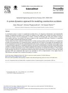
Fig. 3. An example of the time evolution of three worm quasi-species for a case where the IDS is capable of containing the worm’s spread. At each shift a new quasi-species becomes dominant but is unable to attain the concentration of the previous dominant quasi-species before it is detected.
will now have a higher growth rate as compared to the earlier dominant strain. In other words, the fitness landscape for the worm moves. From Equations (17), (18) and (19) we note that a member of the quasi-species group 1 will now have the next highest growth rate. The polymorphic worm adapts to this change in the fitness function on a timescale τw , the time required for the population of the new dominant strain to overtake that of the old. The IDS system now tries to adapt to this new dominant quasi-species and we denote the time required for it to detect the new dominant quasi-species by τids . Through the iteration of the steps above, the worm scours through the sample space of quasi-species and the IDS system follows on its heels. Note that the iteration repeats every τ = τw + τids seconds. If τids is large, the IDS moves slowly and the new dominant strain reaches or exceeds the concentration of the previous dominant strain and the worm will survive for all time. If however the new dominant strain cannot regenerate fast enough (or equivalently, the IDS is fast enough) the new dominant quasi-species will be detected and consequently a shift in the worm’s fitness landscape will occur before it reaches the population level of the previous dominant strain. The next dominant quasi-species will not be able to reach the concentration level of the previous dominant quasi-species and so on. This continues till there is no discernible worm presence in the network. This pattern of chaining quasi-species concentrations is shown in Figure 3. We now determine the required growth rate of the new dominant quasi-species over a full cycle τ as a criterion for the quasi-species’ survival. Consider time t = 0 at the instant when the fitness landscape shifts and an arbitrary quasi-species from the 1st quasi-species group becomes dominant. Using Equation (18) the normalized growth of this quasi-species over a period τ is then given by n
¤ e(1−ǫ) βητ £ w1a (τ ) = 1 + nβηǫ(1 − ǫ)n−1 τ a w1 (0) n(S − 1)
(25)
The quasi-species w1a is currently the fittest. But if another
quasi-species far away from the fitness peak is able to surpass its population in the interval τ , then the currently dominant quasi-species will die out. With the current dominant quasispecies being from the quasi-species group 1 and the quasispecies group 0 having already been detected, we turn to an arbitrary member of the quasi-species group n, wna , since it has the largest Hamming distance from the master sequence. Using Equation (19), its normalized growth rate is then given by n wna (τ ) = eβη(1−ǫ) τ (26) wna (0) The ratio of these growth rates is then k=
w1a (τ ) w1a (0) a (τ ) wn a (0) wn
=
1 + nβηǫ(1 − ǫ)n−1 τ n(S − 1)
(27)
⇒
⇒ ⇒
n
n
w1a (τ ) = e(1−ǫ) (βη−δ)τw w0a (τ ) n n 1 + nβηǫ(1 − ǫ)n−1 τ e(1−ǫ) βητw e(1−ǫ) βητ w0 (0) n(S − 1) n n = e(1−ǫ) (βη−δ)τw e(1−ǫ) βστ w0 (0) 1 + nβηǫ(1 − ǫ)n−1 τ e−δτw = n(S − 1) ¶ µ n(S − 1) 1 (28) τw = ln δ 1 + nβηǫ(1 − ǫ)n−1 τ βητw
τ
= τw +µτids ¶ n(S − 1) 1 + τids ln = δ 1 + nβηǫ(1 − ǫ)n−1 τ 1 1 LamW(x) − = δ nβηǫ(1 − ǫ)n−1
(29)
where x is given by n−1
x=
δ(1+nβηǫ(1−ǫ) τids ) δ(S − 1) nβηǫ(1−ǫ)n−1 e n−1 βηǫ(1 − ǫ)
(30)
and LamW(·) is the Lambert W function, i.e., a function which satisfies LamW(y)eLamW(y) = y (31) Now, solving k < 1 using Equation (27) for τ , we obtain
The quasi-species will die out if k < 1 and survives only when k ≥ 1. 1) Obtaining τw and τids : In order to obtain the maximum allowable limit on τids , we first obtain τw and substitute it in Equation (27). Consider the situation when the IDS system detects the original dominant quasi-species and exerts a kill rate of δ on it. To estimate the timescale for the shift in the worm’s fitness landscape, τw , we first iterate the quasispecies propagation model for a full cycle of length τ starting at t = 0. The switch in the dominant quasi-species is made at t = τ when the IDS starts applying the decay rate of δ on the previous dominant quasi-species. The relative sizes of the new and old dominant quasi-species are then determined for another interval τw and the timescale τw is given by the waiting time until the new dominant quasi-species population exceeds the old one. Note that the populations of the old and new dominant quasi-species as the end of τ are given by w0a (τ ) and w1a (τ ) in Equations (17) and (18) respectively. In the subsequent interval τw , the growth rates of the old and n n new dominant quasi-species are e(1−ǫ) ηβ−δ and e(1−ǫ) βη respectively. Equating the populations of the old and new dominant quasi-species at τw and using w0a (0) = w1a (0) i.e. equal initial conditions, we obtain e(1−ǫ)
allowable IDS response time. Using Equation (28), we can write τ as
where we need n(S − 1) > 1 + nβηǫ(1 − ǫ)n−1 τ for τw to be positive. To find the maximum allowable τids , we note that the worm population dies out and its spread is contained if k < 1 in Equation (27). Thus by substituting τ = τw + τids in Equation (27) and solving for τids we can obtain the maximum
1 + nβηǫ(1 − ǫ)n−1 τ