Intelligent Control and Automation, 2011, 2, 8-23 doi:10.4236/ica.2011.21002 Published Online February 2011 (http://www.SciRP.org/journal/ica)
Unified Modeling Approach of Kinematics, Dynamics and Control of a Free-Flying Space Robot Interacting with a Target Satellite Murad Shibli Mechanical Engineering Department, College of Engineering, United Arab Emirates University, Al-Ain, UAE E-mail:
[email protected] desired Received November 28, 2010; revised December 12, 2010; accepted December 13, 2010
Abstract In this paper a unified control-oriented modeling approach is proposed to deal with the kinematics, linear and angular momentum, contact constraints and dynamics of a free-flying space robot interacting with a target satellite. This developed approach combines the dynamics of both systems in one structure along with holonomic and nonholonomic constraints in a single framework. Furthermore, this modeling allows considering the generalized contact forces between the space robot end-effecter and the target satellite as internal forces rather than external forces. As a result of this approach, linear and angular momentum will form holonomic and nonholonomic constraints, respectively. Meanwhile, restricting the motion of the space robot end-effector on the surface of the target satellite will impose geometric constraints. The proposed momentum of the combined system under consideration is a generalization of the momentum model of a free-flying space robot. Based on this unified model, three reduced models are developed. The first reduced dynamics can be considered as a generalization of a free-flying robot without contact with a target satellite. In this reduced model it is found that the Jacobian and inertia matrices can be considered as an extension of those of a free-flying space robot. Since control of the base attitude rather than its translation is preferred in certain cases, a second reduced model is obtained by eliminating the base linear motion dynamics. For the purpose of the controller development, a third reduced-order dynamical model is then obtained by finding a common solution of all constraints using the concept of orthogonal projection matrices. The objective of this approach is to design a controller to track motion trajectory while regulating the force interaction between the space robot and the target satellite. Many space missions can benefit from such a modeling system, for example, autonomous docking of satellites, rescuing satellites, and satellite servicing, where it is vital to limit the contact force during the robotic operation. Moreover, Inverse dynamics and adaptive inverse dynamics controllers are designed to achieve the control objectives. Both controllers are found to be effective to meet the specifications and to overcome the un-actuation of the target satellite. Finally, simulation is demonstrated by to verify the analytical results. Keywords: Free-Flying Space Robot, Target Satellite, Servicing Flying Robot, Adaptive Control, Inverse Dynamic Control, Hubble Telescope
1. Introduction Free-flying space robots and free-floating space robots have been under intensive consideration to perform many space missions such as: inspection, maintenance, repairing and servicing satellites in earth orbit. Particularly, servicing satellite equipped with robot arms can be employed for recovering the attitude, charging the exhausting batteries, attaching new thrusters, and replacing the Copyright © 2011 SciRes.
failed parts like gyros, solar panels or antennas of another satellite. There are two major classes of space robots can be classified: 1) free-flying space robots and 2) free-floating space robots. The manipulator system of the first type is a system in which the reaction jets (thrusters) are kept active so as to control the position and attitude of the systems’ spacecraft. In opposition to the free flying robot, a free-floating space robotic system is a system in which ICA
M. SHIBLI
the spacecrafts’ reaction thrusters are shut down to conserve attitude control fuel. Comprehensive understanding of the kinematics and momentum of space robots and their interaction with a floating object is considered as a very essential part in designing an efficient multi-body system with effective control techniques of contact forces and motion trajectories. Many techniques in dynamic modeling of space robots have been developed in [1-10]. Kinematics motion of a space robot system are developed based on the concept of a Virtual Manipulator (VM) [10-14]. It assumes imaginary mechanical links and it does not model the angular momentum, then the attitude motion of the base satellite has to be considered by other means. One body of the space robotic system is used as the reference frame with a point on it to represent the transitional DOF of the system [2,8,9]. A tree topology of open chain multi-body system with the system center of mass as the translational DOF is proposed in [6,7]. Many techniques in dynamic modeling of space robots have been reviewed in [2,4,5]. Newton-Euler dynamic approach of multi-body systems is proposed in [6,7]. This approach is characterized the use of a tree topology of open chain multi-body system with the system Center of Mass as the translational DOF. Barycenters are used efficiently to formulate the kinematics and dynamics of free-floating space robots. Another approach is called the direct approach and it uses one body of the system to be the reference frame with a point on it to represent the transitional DOF of the system [2,8,9]. This approach is simpler but results in coupled equations. A virtual manipulator is proposed in [10-14] and used to simplify the system dynamics of space robots. It decouples the system Center of Mass transactional DOF. Free-flying space robots dedicated for maintenance or rescue operations are involved in contact tasks. Many studies on space-based robotic systems have assumed zero external applied forces. Dynamics of space robots by using what is so-called the virtual manipulator (VM) is proposed in [10-14]. Multi-body systems approach based on Newton-Euler dynamic is proposed in [6,7]. Achievements in Space Robotics are presented in [15]. In this article three parts are introduced. In the first part, the achievements of orbital robotics technology in the last decade are reviewed, highlighting the Engineering Test Satellite (ETS-VII) and Orbital Express flight demonstrations. In the second part, some of the selected topics of planetary robotics from the field robotics research point of view are described. Finally, technological challenges to asteroid robotics are discussed. In work [16] three dynamical models of a two link space robot are developed. One model treats the gravitational field as constant over the volume of the robot and Copyright © 2011 SciRes.
9
another model uses 0th order Taylor series expansions of a continuous gravitational field over the volume of the robot. A third model neglects the effects of gravity. The dynamics of a dual-arm space robot system was systematically studied, and a dynamic model based on Kane-Huston’s method and screw theory was presented in [17]. The numerical example shows that acting moment of a composition unit of the robot can be solved for given value of motion parameters with the exploitation of the dynamic model, vice versa. A simulation system of a three layer structure based on ADAMS, MATLAB and VC++ is present in [18], which can simulate and analyze the kinematics and dynamics of space robot in the process of capturing and releasing space object. Verification results show that this system can well explain space robot’s dynamic and kinetic characteristic in capturing and releasing task under the space circumstances. In research [19], the kinematics and dynamics of freefloating coordinated space robotic system with closed kinematic constraints are developed. An approach to position and force control of free-floating coordinated space robots with closed kinematic constraints is proposed for the first time. Unlike previous coordinated space robot control methods which are for open kinematic chains, the method presented here addresses the main difficult problem of control of closed kinematic chains. The controller consists of two parts, position controller and internal force controller, which regulate, respectively, the object position and internal forces between the object and end-effectors. The inverse kinematic control based on mutual mapping neural network of free-floating dual-arm space robot system without the basepsilas control is discussed in [20]. With the geometrical relation and the linear, angular momentum conservation of the system, the generalized Jacobian matrix is obtained. Based on the above result, a mutual mapping neural network control scheme employing Lyapunov functions is designed to control the end-effectors to track the desired trajectory in workspace. The control scheme does not require the inverse of the Jacobian matrix. A planar dual-arm space robot system is simulated to verify the proposed control scheme. In [21], the kinematics of the FFSR is introduced firstly. Then the null space approach is used to reparameterize the path: the direction and magnitude are decoupled and no direction error is introduced. And the Newton iterative method is adopted to find the optimal magnitude of the joint velocity. A planar FFSR with a 2 DOFs manipulator is selected to test the algorithm and simulation results illustrate that the path following is realized precisely. The genetic algorithm with wavelet approximation is applied to nonholonomic motion planning in [22-25]. The problem of nonholonomic motion planning is formulated as an opICA
10
M. SHIBLI
timal control problem for a drift. The problem of position control of robotic manipulators both nonredundant and redundant in the task space is addressed in [26]. A computationally simple class of task space regulators consisting of a transpose adaptive Jacobian controller plus an adaptive term estimating generalized gravity forces is proposed. The Lyapunov stability theory is used to derive the control scheme. In [27] global randomized joint-space path planning for articulated robots that are subjected to task-space constraints is explored. This paper describes a representation of constrained motion for joint-space planners and develops two simple and efficient methods for constrained sampling of joint configurations: tangent-space sampling (TS) and first-order retraction (FR). In work [28], controlmoment gyroscopes (CMGs) are proposed as actuators for a spacecraft-mounted robotic arm to reduce reaction forces and torques on the spacecraft base. With the established kinematics and dynamics for a CMG robotic system, numerical simulations are performed for a general CMG system with an added payload. In [29] the problem of dynamic coupling and control of a space robot with a free-flying base is discussed, which could be a spacecraft, space station, or satellite. The dynamics of the system systematically and demonstrate nonlinearity of parameterization of the dynamics structure is formulated. The dynamic coupling of the robot and base system is studeid, and propose a concept, i.e., coupling factor, to illustrate the motion and force dependencies. Dynamics and control of a flexible space robot capturing a static target was presented in [30]. The dynamics model of the robot system is derived with Lagrangian formulation. The control method of flexible space during capturing target was discussed. Work [31] proposes an adaptive controller for a fully free-floating space robot with kinematic and dynamic model uncertainty. In adaptive control design for the space robot, because of high dynamical coupling between an actively operated arm and a passively moving end-point, two inherent difficulties exist, such as non-linear parameterization of the dynamic equation and both kinematic and dynamic parameter uncertainties in the coordinate mapping from Cartesian space to joint space. Research [32] addresses modeling, simulation and controls of a robotic servicing system for the hubble space telescope servicing missions. The simulation models of the robotic system include flexible body dynamics, control systems and geometric models of the contacting bodies. These models are incorporated into MDA’s simulation facilities, the multibody dynamics simulator “space station portable operations training simulator (SPOTS)”. Most previous studies describing the dynamics of a space robot neglect the coupled dynamics with a floating Copyright © 2011 SciRes.
environment or consider only abstract external forces/ moments or impulse forces. The target has its own inertial and nonlinear forces/moments that significantly influence the ones of the space robot and cannot be ignored. Applying improper forces at the constraint surface may cause a severe damage to the target and/or to the space robot and its base satellite or cause the target to escape away. To accomplish a capture in practice is not instantaneous, because the end-effecter needs to keep moving and applying a force/moment on the surface of the target until the target is totally captured. Moreover, from trajectory planning point of view, not all trajectories and displacements (velocities) are allowed due to the conservation of momentum and geometric constraints. In this work, a unified control-oriented modeling approach is proposed to deal with the kinematics, constraints and dynamics of a free-flying space robot interacting with a target satellite. This model combines the dynamics of both systems together in one structure and handles all holonomic and nonholnomic constraints in a single framework. Moreover, this approach allows considering the generalized constraint forces between the space robot end-effecter and the target satellite as internal forces rather than external forces. Most of the adaptive control algorithms assume the absence of external forces acting on space robot. As it can be seen most studies ignored considering constraints imposed by linear momentum, angular momentum, and contact constraints all together. The kinematics, dynamics, the uncertainty of parameters of a free-flying space robot and that of the target are considered separately. In this paper the uncertainty of the combined system as a whole is considered which gives more global results. In this paper a unified control-oriented dynamics model is developed by unifying dynamics of the spacerobot and the target satellite together along with all holonomic and nonholonomic constraints. Many space missions can benefit from such a control system, for example, autonomous docking of satellites, rescuing satellites, and satellite servicing, where it is vital to limit the contact force during the robotic operation. It worthy to monition that the advantage of this approach is considering the contact forces between the space robot end-effector and the target as internal forces rather than external forces. In this paper, inverse based-dynamics and an adaptive inverse based-dynamics controllers are proposed to handle the overall combined coupled dynamics of the based-satellite servicing robot and the target satellite all together with geometric and momentum constraints imposed on the system. A reduced-order dynamical model is obtained by finding a common solution of all constraints using the concept of orthogonal projection matrices. The proposed controller does not only ICA
M. SHIBLI
show the capability to meet motion and contact forces desired specifications, but also to cope with the underactuation problem [33,34]. The paper is organized as follows: In Section 2, modeling of kinematics, linear and angular momentum, and contact constraints are derived, and then a common solution for all constraints is proposed. In Section 3, an overall dynamics model is developed. In Section 4 an inverse dynamics controller is proposed. An adaptive inverse dynamics controller is presented In Section 5. Meanwhile, in Section 6, simulation results are demonstrated to verify the analytical results, and finally in 7 summary is concluded.
11
We assume that all system bodies are rigid, the contact surfaces are frictionless and known. Also the effect of gravity gradient, solar radiation and aerodynamic forces are weak and neglected. It is assumed also that the base satellite is reaction-wheel actuated. Referring to Figure 1, the position vector of the ith body centroid with respect to the inertial frame can be expressed as
R= Rb + Ri b i
where the relative vector Ri/ b is the position of the ith body centroid with respect to the base frame [35,36]. Upon differentiating both sides of (1) with respect to time, the relationship between the ith body velocity
2. Kinematics and Momentum Modeling 2.1. Nomenclature All generalized coordinates are measured in the inertial frame unless another frame is mentioned as follows mi : the mass of the ith body I i ∈ R 3 : the inertia of the ith body q ∈ R n : the robot joint variable vector q (q1 , q2 , , qn )T Rb ∈ R 3 : the position vector of the centroid of the base RT ∈ R 3 : the position vector of the target satellite centroid ri ∈ R 3 : the position vector of the i-th joint RT/ EE ∈ R 3 : the relative position vector of the target satellite centroid with respect to the end-effecter (EE) Vb ∈ R 3 : the linear velocity of the base Ωb ∈ R 3 : the base angular velocity vector U 3 : the 3 × 3 identity matrix
V= Vb + Ωb × Ri b + vi i
vi = J Li q
(
f bT ,ηbT
)
T
(3)
where J Li = z1 × ( Ri − r1 ) , z2 × ( Ri − r2 ) , , zi × ( Ri − ri ) , 0, , 0
(4)
Link n On qn
Oi + 1 qi + 1
Link i
τ ∈ R : the joint torque vector (τ 1 ,τ 2 , ,τ n ) Fb ∈ R 6 : forces and moments
(2)
where vi is the linear velocities of the ith body in base coordinates. Now in the case of any ith body of the manipulator, the velocity vi can be expressed in terms of the linear Jacobian matrix as
T
n
(1)
On + 1
RT EE
qh
ΣT
Oi qi
act on the
centroid of base satellite.
2.2. Kinematics The purpose of this part is to model the kinematics of a free-flying space robotic manipulator in contact with a captured satellite as a whole. In this model the contact between the space robot and the target satellite is assumed established and not escaped. Our combined system can be modeled as a multi-body chain system composed of n + 2 rigid bodies. While the manipulator links are numbered from 1 to n, the base satellite (body 0) is denoted by b, in particular, and the ( n + 1) th body (the target satellite) by T. Moreover, This multi-body system is connected by n + 1 joints, which are given numbers from 1 to n + 1. Where the end-effecter is represented as the ( n + 1) th joint as shown in Figure 1. Copyright © 2011 SciRes.
O3
ΣCG
q3
Ri b Link 2 q2 O2 q1
Link 1 O1
ΣB
ΣI
Figure 1. Free-floating space robot in contact with a target satellite.
ICA
M. SHIBLI
12
where each block of the matrix is defined as follows
The end-effecter tip velocity is given by
VEE= Vb + Ωb × REE b
+ J LEE q
n +1
(5)
M Vb ≡ U 3 ∑ mi ∈ R 3×3
Additionally, the velocity VT of the target satellite in the reference frame can be obtained by deriving Equation (1) as (6) VT= Vb + Ωb × RT b + J LT q + ωT × RT EE + vT
M Vb Ωb ≡ −
=i
M Vb q ≡
Since the target satellite is not stationary, (6) shows the relative linear and angular velocities vT , ωT between the end effecter and the target satellite and measured in the base frame. Another relationship is needed between the ith body angular velocity Ωi and joint angular velocity
Ωi =Ωb + ωi
(14)
i =0
M Ωb ≡
mi Ri × ∈ R 3×3 /b 0, i ≠ b
n +1
∑
mi J L ∈ R 3×n
n +1
{I + m D( R )} + I
=i 0, i ≠ b
∑
=i 0, i ≠ b
M Ωb q ≡
(7)
n +1
∑
n +1
∑
=i 0, i ≠ b
(15) (16)
i
i
i
{ IJ B
i
Ai
i/ b
b
∈ R 3×3
}
+ mi Ri/ b × J L ∈ R 3×n i
(17) (18)
where ωi is the angular velocities of the ith body in base coordinates and ωi in case of the manipulator is given by (8) ωi = J Ai q
M VbωT ≡ −mn+1 RT/ EE × ∈ R 3×3
M Vb vT ≡ U 3 mn +1 ∈ R 3×3
(21)
where the angular Jacobian
M Ωb vT ≡ −mn+1 [ Rn +1 ×] ∈ R 3×3
(22)
J Ai = [ z1 , z2 , , zi , 0, , 0]
/ EE
(9)
While in the case of the target satellite, the absolute angular velocity of can be expressed as
ΩT =Ωb + J AT q + ωT
M ΩbωT ≡ mi D( RT
0 [ R ×] ≡ Rz − Ry
Former analysis will be used in the next analysis to derive the momentum of s free-flying space robot.
(11)
i =0
i =0
(
B
I i Ωi + mi Ri × Vi
)
(12)
By means of (2-10), linear and angular momentum in (11-12) can then be represented in a compact form as
P = L
M Vb Ωb Vb M Vb q M Vb T + q M VbΩb M Ωb Ωb M Ωb q (13) M VbωT M Vb vT ωT + M ΩbωT M Ωb vT vT
Copyright © 2011 SciRes.
for a vector
Ry − Rx ∈ R 3×3 0
(23)
T
n +1
n +1
[ R ×]
D ( R ) ≡ [ R ×] [ R ×]
The linear and angular momentum of a multi-body system is a key part in understanding the motion of the system when it is not subjected to external forces. They may impose kinematic-like constraints when the system is free of any external force. The linear momentum P and angular momentum L of the whole system is given by
L≡∑
− Rz 0 Rx
(20)
and
2.3. Linear and Angular Momentum
P ≡ ∑ miVi
) + b I n +1 ∈ R 3×3
Note that the matrix function T R = Rx , Ry , Rz is defined as
(10)
(19)
Ry2 + Rz2 = − Rx Ry − Rx Rz
− Rx Ry Rx2 + Rz2 − Ry Rz
− Rx Rz (24) − Ry Rz ∈ R 3×3 Rx2 + Ry2
and the sub-matrices of the Jacobian of the ith body representing the linear and angular parts are defined before. Note that as in (13) the system is subjected to a nonholonomic (non-integrable) constraint because of conservation of angular momentum in the absence of external forces. Note that the momentum constraints are not purely kinematical because of the inertial characteristics it carries in. Thus, this constraint is called kinematicslike. The physical meaning behind these constraints is that they restrict the kinematically possible displacements (possible velocities) of the individual parts of the system. On the contrast, the linear momentum results in a holonomic (integrable) constraint. Now assuming zero initial conditions then linear and angular momentum is give by ICA
M. SHIBLI
0 0
M Vb Ωb Vb M Vb q M Vb T + q M VbΩb M Ωb Ωb M Ωb q M VbωT M Vb vT ωT + M ΩbωT M Ωb vT vT
2.5. Common Solution of the Constraints (25)
Then it is possible that the relative linear and angular velocities of the target satellite can calculated as
M VbωT ωT v = − M T ΩbωT M VbωT − M ΩbωT
−1
M Vb vT M Vb T M Ωb vT M VbΩb M Vb vT M Ωb vT
−1
M Vb Ωb Vb M Ωb Ωb
M Vb q q M Ωb q
(26)
2.4. Contact Constraints We assume that the end-effecter moves on a sub-surface of the target satellite S and the profile of this surface is known so that it can be defined as (27)
Let χ be the vector of generalized coordinates of the robot end-effecter in the target frame. The end-effecter, as a result of the contact with the target, is subjected to holonomic kinematic constraints defined in the constraint frame as
Φ(χ ) = 0
(28)
where Φ (⋅) : R n → R m is twice differentiable. The robot joint and target coordinates are related through the forward kienmatic function
χ = f (q)
(29)
Now differentiating (28) with respect to time gives
∂Φ ( χ ) ∂χ
χ = 0
∂f ( q ) ∂q
(30)
q
(31)
Substituting (31) into (30) (chain rule) yields to
∂Φ ( χ ) ∂f ( q ) ∂χ where the matrix Jθ = matrix Copyright © 2011 SciRes.
∂q
q = 0
∂Φ ( χ ) ∂f ( q ) ∂χ
∂q
(33)
where Jθ (θ ) is the Jacobian of the holonomic constraint as defined in (32). On the other hand, the conservation of momentum holds two types of constraints: linear momentum which is holnomic; and nonholnomic constraints come into play as a result of the conservation of the angular momentum. These momentum constraints are not given in algebraic form, but there are given in kinematical-like form as in (13) and can be rewritten in a compact form as
B (θ ) θ = c0
(34)
where c0 represents the vector of the initial conditions of the momentum. Equation (34) has k momentum constraint equations with k ≤ N , where N is number of generalized coordinates. The purpose of representing holonomic constraints in the form (33) is to treat both holonomic and nonholonmic constraints at the same differential level. But a difference exists in the matter of initial conditions. Holonomic constraints are restricted to position initial conditions, but nonholonomic are only restricted to their momentum conditions. Now, all holonomic and nonholonomic constraints can be combined together as
Jθ (θ ) 0 θ = c0 B (θ )
(35)
(32)
{ N ( Jθ )} {B c + N ( B )} +
is the Jacobian
T
where the new combined matrix Jθ (θ ) B (θ ) is of dimension ( k + m ) × ( n + 1) . This implies a set of ( k + m ) linear equations with θ as vector of the generalized variables. Since matrices Jθ (θ ) and B (θ ) have the same number of columns, we now seek for their common solutions, if exist, expressing them in terms of the solutions of (33) and (34). The common solutions of (33) and (34) are the solutions of the combined constraints (35). From the theory of linear algebra, the solutions of Equations (33) and (34) constitute the intersection manifold T
Also differentiating (29) with respect to time
χ =
In this section we study the constraints on a space robot in contact with a target satellite in one form. This entire system is subjected to holonomic and nonholonomic constraints at the same time. These Holonomic constraint are usually given in algebraic form relating the generalized variables (28). Now differentiating the holonomic constraint at the velocity level as in (30-32) leads to
Jθ (θ ) θ = 0
Equations (26) enables us to calculate the target velocities [ωT vT ] without measurements.
S : F ( x, y, z , α , β , γ )= c= const.
13
T
(36)
where N ( Jθ ) and N ( B ) are the null space of Jθ and B, respectively. And the upper right script + ICA
M. SHIBLI
14
represents the Pseudoinverse. Equation (36) is the set of solutions of (33) and (34) is consistent if (36) is nonempty. Then the common solution [36] is the manifolds
(
(a) PN ( Jθ ) PN ( Jθ ) + PN ( B )
)
+
B + c0 + N ( Jθ ) + N ( B ) (37)
(
B + c0 − PN ( B ) PN ( Jθ ) + PN ( B ) (b) =
)
+
B + c0
(38)
+ N ( Jθ ) + N ( B )
(
(c) = Jθ+ Jθ + B + B
)
+
B + c0 + N ( Jθ ) N ( B )
(39)
(
(d) X = Jθ
0 + PN ( Jθ ) PN ( Jθ ) + PN ( B )
)
+
(
(e) Y = 0 B − PN ( B ) PN ( Jθ ) + PN ( B ) +
− Jθ
B +
)
+
− Jθ
+
B +
(41) ( f) Z =
(J
θ
+
Jθ + B B
)
+
Jθ
+
B +
(42)
( )
( )
R Jθ ∗ R B∗ = {0}
(43)
then each expressions of (40-42) is the Moore-Penrose T
T T inverse of Jθ (θ ) B (θ ) .
3. Generalized Dynamics Modeling To drive the dynamic equation of a space robot interacting with a target, the total system kinetic energy as the total summation of the transitional and rotational energy of each body in the system can be expressed as
1 n +1 ∑ miViT Vi + ΩTi b Ii Ωi 2 i =0
(
)
(44)
where Vi and Ωi is the transitional and rotational velocities of i-th body , respectively, or it can be rearranged
= T
M Ωb
M Ωb q
M ΩbωT
M ΩT q
Mq
M qωT
T
T
b
MΩ ω
M qω
T
M ωT
M ΩT v
M Tqv
T
M ωT v
b T
bT
M Vb vT M Ωb vT M qvT M ωT vT M vT
T T
Vb Ω b q ωT vT
where the block matrix in (45) is the inertia matrix and the sub-matrices are defined previously in (14-22) and also
Mq ≡
n +1
∑ {mi J LiT ⋅ J L
i
=i 0, i ≠ b
}
+ B I i J TAi J Ai ∈ R (
n +1)×( n +1)
(46)
(
M ωT ≡ I n +1 + mn +1 D RT
/ EE
)∈ R
1 [Vb Ωb q ωT vT ] 2
Copyright © 2011 SciRes.
T M qvT ≡ mn +1 J LT U ∈R
3×( n +1)
M ωT vT ≡ −mn +1 RT
× ∈ R 3×3
3×3
(47)
EE
(49) (50)
M vT ≡ U 3 mn +1 ∈ R 3×3
(51)
Note that the inertia matrix M defined in (45) is symmetric positive definite. Now define
θ VbT =
Moreover, if
T≡
M VbωT
(48) +
(40)
+
M Vb q
3× n +1 T T T + mn +1 J LT M qωT ≡ I n +1 J AT R × ∈ R ( ) T EE
T
T B (θ ) : +
M Vb Ωb
(45)
where PN (⋅) is the projection matrix on the null space of a given matrix (⋅) . Since each of the manifolds given in (37)-(39) give a solution of the combined system (35), these expressions can also be used to get the generalized (pseudo-inverse) of the combined matrices. Each of the following expressions is a {1, 2, 4} − inverse of the combined matrix
Jθ (θ )T
M Vb T M VbΩb T × M Vbq M T VbωT M T VbvT
ΩTb
q T
ωTT
vTT
(52)
Then the total kinetic energy can be expresses in a compact from
1 T = θT M (θ ) θ 2
(53)
From the kinetic energy formulation, the dynamics equations can be derived by using the Lagrangian approach. Since there is no potential energy accounted in our system, the Lagrange function L is equal to the kinetic energy T then becomes
d ∂T ∂T − = τ + JTλ dt ∂θ ∂θ
(54)
where λ is the vector of unknown Lagrangian multipliers. The holonomic constraints are behind the generalized constraint forces as a result of the contact between the manipulator end-effecter and the surface of the target satellite. The combined system dynamics model can be represented as (assuming the target satellite is unactauted) ICA
M. SHIBLI
M Vb T M VbΩb T M Vbq M T VbωT MT VbvT
M Vb Ωb
M Vb q
M VbωT
M Ωb
M Ωb q
M ΩbωT
M ΩT q
Mq
M qωT
T
T
b
MΩ ω
M qω
T
M ωT
M ΩT v
M Tqv
T
M ωT v
b T
bT
T FbL J bL F JT bA bA T = τ + Jθ T 0 J TwT 0 J T TvT
T T
M Vb vT CV0 Vb M Ωb vT C Ω Ωb b M qvT q + Cq M ωT vT ωT CwT M vT vT CvT
λ
full rank and belong to the null space of A ( q ) and the vector ν ∈ R ( N − k − m ) can be chosen arbitrary. It implies that S T A = 0 . [37] Now differentiating (57) at the acceleration level with respect to time yields
= θ Sν + Sν
(58)
Upon substituting the velocities (57) and the acceleration (58) into the dynamics (55) we obtain
(
)
MSν + MS + CS ν =+ τ Fc
(59)
Let us define the controller as τ
τ = ( HS + CS )ν + HS (νd + K D e + K P e ) − J T λc (60)
(55) The dynamic developed in (55) along with the combined constraints in (35) completes the overall modeling of a space robot interacting with a target satellite.
4. Inverse Dynamics Control The basic idea of inverse dynamics control is to seek a nonlinear dynamics control law that cancels exactly all nonlinear terms in the system dynamics (55) so that the closed loop dynamics is linear and decoupled [6]. Now assuming zero initial conditions in (13) and (35), the overall dynamics subjected to the constraints can be expressed in a compact form as
M θ + Cθ = τ + Fc
(56)
where the inertia matrix M is defined in (55), the nonlinear vector C θ , θ is the centrifugal/Coriolos forces the generalized constraint forces are Fc = J T λ , λ ∈ R m is the vector of unknown Lagrangian multipliers, J T and τ are defined, respectively, as T J bL FbL T J bA FbA T T J = J q , τ = τ as in (55), and finally the T J Twt 0 T J Tvt 0
(
15
)
J (θ ) constraint matrix A (θ ) = θ as given in (35). B (θ ) In the constraint Equation (35) there are ( k + m ) linear equations and N of the generalized velocities θ . It clear that there are fewer equations than unknowns, this implies the existence of infinite solutions. From the theory of linear algebra, the solution of (35) can be given by (57) θ = S (θ )ν
where S (θ ) ∈ R ( N )×( N − k − m ) is an orthogonal projector of Copyright © 2011 SciRes.
where the position tracking error is defined as e= ν d −ν and λc is defined as p
λc = λd − K F eF − K I ∫ eF dt
(61)
where eF= λ − λd and the gain matrices K P , K D , K F and K I are chosen as diagonal with positive elements. Note that the input to the proposed controller (60) are the joint angles and velocities, angular velocity of the base, relative velocities of both satellites, contact forces and the output of the controller is the joint torques. Note also that sT τ ∈ R N − k − m has the advantage of overcoming the underactuation of the system as a result of target satellite jet shutdown or failure, and the inputs provided by the robot and the base is enough to control the whole system. This is because the number of constraints k + m ≥ the number of passive inputs of the target satellite. Now let us substitute the control law (60) into the dynamics (59), then, the closed loop dynamics is given by
S T MS ( ep + K D e p + K P e p )
(
= − S T J T K F eF + K I ∫ eF dt
)
(62)
=0 Since J belongs to the null space of S, that is, S T J T = 0 and since by the virtue of (57), the projection matrix S ( q ) and its transpose are of full rank, and the inertia matrix is symmetric positive definite, then S T MS is also a positive definite. Now we need to verify the terms inside the brackets in (60) are zero. This condition can be guaranteed by choosing the proper positive gains K D and K P such that ν → ν d as t → ∞ . If the gain matrices K D and K P are chosen as diagonal with positive diagonal elements, then the resulted closed loop dynamics is linear, decoupled and exponentially stable. Global stability can then be guaranteed. The closed loop dynamics natural frequency and damping ration can be chosen to meet specific requirements. Also ICA
M. SHIBLI
16
Hˆˆ1ν − H1ν + H1ν + C1ν = Hˆ 1 (νd + K D e + K P e ) + Cˆ1ν − S T J T ( λc − λ )
by inspecting the right hand side we can see that the
K F eF + K I ∫ eF dt can be guaranteed to be zero by choosing the suitable gain matrices K F and K I . Now we can readily summarize the hybrid inversedynamics controller in the following theorem: Theorem 1: For the dynamic system given in (59) and subjected to constraints (35), the inverse dynamics control law defined by (60)-(61) is globally stable and guarantees zero steady state and force tracking errors. To further improve the dynamic response in case of system parameters uncertainty, an adaptive controller would serve that objective as in the nest section.
Similar to the analysis followed in the previous section and recalling (60)
(
)
(63)
Now we assume that there are some uncertainties in the system parameters such as masses and inertias and for this reason an adaptive control approach will be investigated. The dynamics (63) can be represented by benefiting from the property of linearity in parameters as [38,39]
H1ν + C1ν = Υα
(
(64)
)
where H1 = HS , = C1 HS + CS , Y is an N × ( N − m ) matrix of known functions and known is the regressor, and α is an ( N − m ) -dimensional vector of the system parameters. After examining the structure of dynamics (55), three properties are obtained: Property 1: T The modified inertia matrix H 2 = S (θ ) H (θ ) S (θ ) is symmetric positive definite. Property 2: If Property 1 is verified, then ( H 2 − 2C2 ) is skew-symmetric matrix where C2 = S T C1 . Property 3: The dynamics (64) is linear in its parameters. The nonlinear control law is proposed to have the form
τ= Hˆ 1 (νd + K D e + K P e ) + Cˆ1ν − J T λc
(65)
where λ= λd − K F eF and K F is a positive definite c diagonal matrix for the force control feedback gain and eF= λ − λd , and where Hˆ 1 and Cˆ1 are the estimates of H1 and C1 , respectively. Note that the geometric of the Jacobian in (56) is assumed to be determined. Then the dynamics (55) can be modified to
Hˆ 1ν + Cˆ1ν = Υαˆ
(66)
where αˆ is the estimated vector of parameters α . Upon substituting (65) into (63), and by adding and subtracting at the same time the term Mˆ 1v on the left hand side of (65) we get Copyright © 2011 SciRes.
Rearranging (58) and canceling out the similar terms, yields
H1ν − Hˆ 1ν + C1ν − Cˆ1ν = Hˆˆ1 (νd −ν + K D eP + K P eP ) − H1ν
(68)
= Y α or,
H 1ν + C1ν= Hˆ 1 ( eP + K D eP + K P eP = ) Y α
(69)
where e= νd −ν , and ( ⋅ ) = ( ⋅) − ( ˆ⋅ ) . The closed loop P dynamics error can be written as
5. Adaptive Inverse Dynamics Control
HSν + HS + CS ν =+ τ JTλ
(67)
Y1α ( eP + K D eP + K P eP ) =
(70)
−1 1
where Hˆ Y = Y1 . It is possible now to express the error dynamics (70) in a state space form as
= x Ax + Bα
(71)
where
e p O ,A x = = − K P e p
I O ,B = −KD Y1
(72)
where A is a Hurwitz matrix, that is, the real parts of its eigenvalues are negative, which guarantees globally exponentially stability. Based on the state space formulation and Lyapunov techniques an adaptive control law can be chosen as
α = −Γ −1Y1T BT Px
(73)
where Γ > 0 and symmetric , and P is a unique positive definite solution to the Lyapunov equation AT P + PA = −Q where Q is a positive definite symmetric. Proof: Let the Lyaponuv candidate function chosen as
V= xT Px + α T Γα
(74)
Now if take the time derivative of V along the trajectories of (71) and by using the adaptation law (65), one gets V= x T Px + xT Px + α T Γα + α T Γα
= ( Ax + BY1α ) Px + xT P ( Ax + BY1α ) T
(
− Γ −1Y1T BT Px
)
T
Γα − α T Γ Γ −1Y1T BT Px
= xT AT Px + α T Y1T BT Px + xT PAx + xT PBY1α
(75)
− x P BY1 Γ Γα − α Γ Γ Y B Px T
(
T
−T
)
T
−1
T 1
T
= xT AT P + PA x + α T Y1T BT Px + xT PT BY1α − xT PT BY1α − α T Y1T BT Px
ICA
M. SHIBLI
By canceling out equivalent terms, this reduces to (76)
Since V is negative semidefinite with regard to x and the parameter error, and V is lower bounded by zero, V remains bounded in the time interval [ 0, ∞ ) . This fact can be stated as ∞
∫0