ERDC TN-SWWRP-11-1 January 2011
A Generic Modeling Approach to Biomass Dynamics of Sagittaria latifolia and Spartina alterniflora by Elly P. H. Best, William A. Boyd, and Kevin P. Kenow
PURPOSE: This technical note describes an ecological modeling approach that can be used to explore relationships between species of emergent aquatic vegetation communities and their environmental conditions. The modeling approach was used to evaluate the potential persistence of two desired — and quantitatively important — rhizomatous plant species under various climatological conditions: Sagittaria latifolia, common in freshwater systems, can produce tubers as well as rhizomes; Spartina alterniflora is typical for coastal marshes. Both species are endemic to the United States. BACKGROUND: Emergent aquatic vegetation may play important roles in aquatic ecosystems. Functions attributed to “desirable” species are: stabilization of sediment and shores, amelioration of water transparency, regulation of nutrient availability in the water column and service as a habitat and food source for invertebrates, fish and waterfowl. Conversely, effects attributed to “nuisance” or “invasive” species are: excessive biomass production that interferes with human utilization of water resources, or displacement of desirable indigenous communities. Distribution and abundance of emergent vegetation in large water bodies in the Mississippi River System (UMRS) and Coastal Louisiana (CL) have changed for decades and declined in recent years. In general, variation in environmental factors such as water depth, temperature, clarity, current, wave action, and substrate characteristics would be expected to affect the distribution and production of emergent macrophytes (Gosselink and Turner 1978). Sagittaria latifolia (Broadleaf arrowhead) is a desired and dominant species in the UMRS, where it provides a significant annual autochthonous input (Eckblad et al. 1977). In this river system, changes resulting from the man-made modification of the hydrologic cycle include installing a system of dams in the 1930s, navigation pools with artificially-maintained high water levels, island loss due to erosion, and increased sedimentation (Bellrose et al. 1979; Eckblad et al. 1977). Environmental changes (such as increased water level and turbidity) resulting from the operation of this navigation system for barge transportation of bulk commodities, have been listed as contributing to the decline of S. latifolia. The latter statement is confirmed by the fact that experimental decreases in water level during the summer growth season in UMRS Pool 5 led to the increased abundance and distribution of emergent vegetation (Kenow et al. 2007). Spartina alterniflora (Smooth cordgrass) is a desired species in CL, where it dominates large portions of the salt marshes because of its high primary production (Kirby and Gosselink 1976; Darby and Turner 2008). Its spatial distribution is limited to the coastal areas along the entire Atlantic and the Southern Pacific seaboards of the United States. Large-scale diebacks have occurred and have been attributed to multiple causes: permanent dieback to prolonged flooding of the subsiding marsh surface (Webb et al. 1995); temporary dieback to drought from which the
Form Approved OMB No. 0704-0188
Report Documentation Page
Public reporting burden for the collection of information is estimated to average 1 hour per response, including the time for reviewing instructions, searching existing data sources, gathering and maintaining the data needed, and completing and reviewing the collection of information. Send comments regarding this burden estimate or any other aspect of this collection of information, including suggestions for reducing this burden, to Washington Headquarters Services, Directorate for Information Operations and Reports, 1215 Jefferson Davis Highway, Suite 1204, Arlington VA 22202-4302. Respondents should be aware that notwithstanding any other provision of law, no person shall be subject to a penalty for failing to comply with a collection of information if it does not display a currently valid OMB control number.
1. REPORT DATE
3. DATES COVERED 2. REPORT TYPE
JAN 2011
00-00-2011 to 00-00-2011
4. TITLE AND SUBTITLE
5a. CONTRACT NUMBER
A Generic Modeling Approach to Biomass Dynamics of Sagittaria latifolia and Spartina alterniflora
5b. GRANT NUMBER 5c. PROGRAM ELEMENT NUMBER
6. AUTHOR(S)
5d. PROJECT NUMBER 5e. TASK NUMBER 5f. WORK UNIT NUMBER
7. PERFORMING ORGANIZATION NAME(S) AND ADDRESS(ES)
U.S. Army Engineer Research and Development Center,System-Wide Water Resources Program (SWWRP).,3909 Halls Ferry Road,Vicksburg,MS,39180 9. SPONSORING/MONITORING AGENCY NAME(S) AND ADDRESS(ES)
8. PERFORMING ORGANIZATION REPORT NUMBER
10. SPONSOR/MONITOR’S ACRONYM(S) 11. SPONSOR/MONITOR’S REPORT NUMBER(S)
12. DISTRIBUTION/AVAILABILITY STATEMENT
Approved for public release; distribution unlimited 13. SUPPLEMENTARY NOTES 14. ABSTRACT
15. SUBJECT TERMS 16. SECURITY CLASSIFICATION OF: a. REPORT
b. ABSTRACT
c. THIS PAGE
unclassified
unclassified
unclassified
17. LIMITATION OF ABSTRACT
18. NUMBER OF PAGES
Same as Report (SAR)
23
19a. NAME OF RESPONSIBLE PERSON
Standard Form 298 (Rev. 8-98) Prescribed by ANSI Std Z39-18
ERDC TN-SWWRP-11-1 January 2011
vegetation could recover rapidly by regrowth from rhizomes or more slowly in the absence of the rhizomes by seedling recruitment in the opened areas (Edwards et al. 2005). Besides light (as affected by water level and turbidity), nitrogen (N) and phosphorus (P) are generally believed to be the most important limiting factors in aquatic systems (Hutchinson, 1975). Relationships between biomass nutrient concentrations and nutrient limitation are complex. Biomass nutrient concentrations tend to be positively correlated with nutrient supply when all other resources are sufficiently available (Guesewell and Koerselman 2002). A low concentration of N in plant biomass should reflect a low availability of N to this plant and, therefore, indicate that additional supply of N would increase the plants’ biomass production. By definition, this means that N is limiting (Vitousek and Howarth 1991). If two or more nutrients (e.g., N and P) are in short supply, their availability relative to each other is likely to determine which of them is limiting. Thus, the molar ratio of N:P, rather than the individual concentrations, should indicate limitation (Koerselman and Meuleman 1996), with tissue N:P ratios less than 14 indicative of N-limited growth in terrestrial plants (Aerts and Chapin 2000). Nutrient-related growth limitation of emergent plants in natural systems has been reported, but N:P ratios have not usually been determined. In S. latifolia, N may limit growth under natural conditions since results of a short-term pot experiment indicated that this plant depleted the exchangeable N in natural sediments within four weeks, but left substantial P levels (Barko et al. 1988; Barko and Smart 1983). In S. alterniflora, it was suggested that N also limits growth under natural conditions, based on the vegetation response to N fertilization in the field (Valiela and Teal 1974; Gallagher 1975). In contrast, the average N:P ratio of 16:1 in aboveground biomass and of 37:1 in belowground biomass suggested P limitation in belowground biomass at this CL site (Darby and Turner 2008). However, growth limitation by nutrient availability may be even more complicated in plants exposed to different salinity levels, as illustrated by the results of a pot experiment in which the critical N:P ratios were determined in S. alterniflora. In these plants, growth was limited by N with tissue N:P ratios ≤13 and aboveground biomass was correlated with interstitial sediment-N concentration, but growth rate was affected by salinity (Smart and Barko 1980). The relationships between the potential persistence of both plant species, nutrient limitation, and salinity have not yet been unequivocally elucidated; consequently, placeholders have been included in the model in anticipation of supporting data. Simulation models that include descriptions of aquatic vegetation responses to changes in physical and chemical conditions in various climates can be valuable tools for water resource managers. These models can be used to evaluate key environmental conditions in which the vegetation would persist or produce excessive biomass, with ensuing consequences for the systems in which they grow. Additionally, the models may provide insight as to how the vegetation would be affected by different management scenarios (Carr et al. 1997; Best et al. 2001; Karunaratne and Asaeda 2002; Asaeda et al. 2008). In this paper, a dynamic simulation modelling approach to emergent plant biomass formation is summarized, with light and temperature as driving variables, and including descriptions of plant responses to human influences such as management measures resulting in changes in turbidity, mechanical harvesting, grazing, and flooding. Calibration of plant responses to current velocity and nutrient limitation will be added later on when calibration values become available. This modelling approach was applied to submersed aquatic vegetation (SAV) also (Best and Boyd 2008). The approach is mathematically similar to those followed in other models for emergent vegetation, such as those developed for Phragmites australis (Ondok 1973; Asaeda and Karunaratne 2000; Asaeda et al. 2008) and for S. alterniflora 2
ERDC TN-SWWRP-11-1 January 2011
(Morris 1989; Dai and Wiegert 1996a). The approach describes plant morphology and biomass formation in relative detail, but it differs from them in that it relates ecophysiological processes to developmental cycle, using the model to simulate plant communities in different climates. In this construct, aerial shoots absorb CO2 from air, and submerged shoots absorb it from water where CO2 availability is assumed to be typical for hard water with an alkalinity between 0 and 300 mg L-1 and a circumneutral pH; effects of changes in CO2 availability are not included. The model species are S. latifolia and S. alterniflora; both plants have similarities in growth strategy, but are significantly different in morphology and physiology. The model has been calibrated, tested for sensitivity and validated against field data for both species. Both species have the capacity to persist in eutrophic, shallow water bodies with fluctuating water levels; both are capable of forming substantial above-and belowground biomass, thereby functioning as important marsh–characteristic elements. Important physiological differences are that S. latifolia fixes carbon via the C3 photosynthetic pathway in contrast to S. Alterniflora, which uses the C4 pathway; S. latifolia has a higher potential photosynthetic rate at light saturation for aerial shoots, and a higher species-characteristic light extinction coefficient than S. alterniflora; S. latifolia can form tubers (i.e., organs), enabling survival during adverse conditions such as drought and cold; S. latifolia is sensitive to increased salinity. These are characteristics which make S. latifolia a species that may predominate in freshwater and coastal marshes with a relatively low salinity, whereas S. alterniflora grows well in coastal marshes of higher salinity. With both species having different strategies to survive adverse conditions, changes in spatial distribution and replacement of one species by the other (the latter in coastal areas only) over a period of one to several years can be expected. Consequently, the described ecological model provides an ideal means to investigate the effects of relatively short-term changes in environmental conditions on the potential persistence of these two emergent species in shallow water bodies as part of restoration plans, provided detailed information on environmental conditions is available. Besides model calibration and validation, two other aspects of the relationship between important representatives of rhizomatous plant species and environmental conditions were investigated in the present study. A dynamic ecological modeling approach was used: (i) persistence at various flood and drought conditions, and (ii) persistence under more southern climatological conditions than at the calibration site. ECOLOGICAL MODELING APPROACH: This ecological model type simulates the carbon flow mass balance of typical emergent vegetation on a 1-m2 sediment/soil with an overlying water column (Figure 1). Growth is considered as the plant dry matter accumulation, including rhizomes, and, if present, subterranean tubers, in an environment where N and P may be limiting under the prevailing weather conditions. At least one plant cohort waxes and wanes per season in different climatological conditions, varying from temperate to tropical. The rate of dry matter accumulation is a function of irradiance, temperature, CO2 availability and plant characteristics. The rate of CO2 assimilation (photosynthesis) of the plant community depends on the radiant energy absorbed by the canopy. The daily rate of gross CO2 assimilation of the community is calculated from the absorbed radiation, the photosynthetic characteristics of leaves and the CO2 availability. Calculations are executed in a set of subroutines added to the model. Part of the carbohydrates produced is used to maintain the existing biomass. The remaining carbohydrates are converted into structural dry matter (plant organs). In the conversion process, part of the weight is lost in respiration. The dry matter produced is partitioned among the various plant organs using partitioning factors, defined as a function of the phenological cycle of the community. The 3
ERDC TN-SWWRP-11-1 January 2011
dry weights (DW) of the plant organs are obtained by integration of their growth rates over time. The plant may over-winter through rhizomes and/or tubers in the sediment without or with plant biomass present. Rhizomes may persist when a critical rhizome mass is maintained. Tubers are depleted and disintegrate in the summer following the season in which they were formed. All calculations are performed on an m2 basis. Since environmental factors and plant growth characteristics vary with plant height and water depth, in the model the growth-related processes of the aboveground plant biomass and the water column have been partitioned in 0.10-m depth layers. A relational diagram is presented in Figure 2. Seed formation has not been included in the model, because its role in maintaining established emergent plant communities in a temperate climate is minimal. Dispersal and colonization of new habitats are recognized, important characteristics of emergent plants. The latter processes, however, are better described using other modelling approaches (based on logistic regression or on descriptions of population dynamics varying in time and space), as described by Scheffer (1991).
Figure 1.
Schematic generic emergent plant growth model.
General features of the model include that it:
Is operational in a one-dimensional (quasi two-dimensional) configuration
Follows a state variable approach
Provides that the state variable selected may be individually activated or deactivated
Performs integration using the Runge-Kutta method
Computes photosynthesis per second and other masses per day
4
ERDC TN-SWWRP-11-1 January 2011
Figure 2.
Relational diagram illustrating the following model processes in ARROW: (1) phonological cycle and development; (2) photosynthesis, respiration, and biomass formation; and (3) flowering, translocation, senescence and wintering organs (the latter process in grey background). Rectangles represent quantities (state variables); valve symbols, flows (rate variables); circles, auxiliary variables; underlined variables, driving and other external variables; dashed lines, information flow (symbols according to Forrester 1961).
5
ERDC TN-SWWRP-11-1 January 2011
Operates as a stand-alone version fitted in a FORTRAN Simulation Environment (FSE) shell (Van Kraalingen 1995). Provides binary and ASCII output files, and graphics that can be viewed within a user-friendly shell. Coded in ANSI Standard FORTRAN F77.
Central Features. Central features of the model are the (1) link between the species-characteristic phenological cycle, physiological processes and environmental conditions and (2) state variable equation determining instantaneous gross photosynthesis. Species-characteristic Phenological Cycle. The phenology of the plant community, for which the development phase can be used as a measure, is modelled as a sequence of processes that take place over a period of time, punctuated by more or less discrete events. The development phase (DVS) is a state variable in the models. The DVS is dimensionless and its value increases gradually within a growing season. The development rate (DVR) has the dimension d-1. The multiple of rate and time period yields an increment in phase. The response of DVR to temperature in the model is in accordance with the degree-day hypothesis (Thornley and Johnson 1990). Calibration, according to this hypothesis, allows use of the model for the same plant species at various sites with different climates (temperature regime). The relationships between the development phase, day-of-year, and 3oC day-degree sum for a temperate climate are presented in Table 1. Each simulation starts at the first Julian day (i.e., 1 January, when the DVS has the value of 0.0). For S. latifolia, a species that may overwinter with rhizomes and tubers, the simulation starts using a selected rhizome weight and/or tuber bank density/individual tuber weight combination as initial values. Initiation of growth activity occurs by sprouting of the tubers, or sprouting of a fixed number of plants at a DVS ≥ 0.292. Sprouts of the first plant cohort develop through remobilization of carbohydrates until the tubers or rhizomes are depleted. If the first plant cohort does not succeed in becoming self-supporting and DVS is less than 1.001, a second cohort sprouts from the tuber bank or rhizomes. For S. alterniflora, a species that overwinters with rhizomes, the simulation starts using a selected rhizome weight. The DVS values of the phenological processes in S. alterniflora differ from those in S. latifolia (Table 1). Instantaneous Gross Photosynthesis and Biomass Formation. Light availability is an important factor influencing the distribution and abundance of aquatic plants. For emergent leaves, light attenuation only within the plant canopy occurs. Leaves submersed in water may have a small part of the irradiance reflected by the water surface, and further attenuation may occur by water and its suspended solids and by the plant itself, either covered by epiphytes or not. Emergent leaves fix carbon with a higher potential photosynthetic rate at light saturation than submersed leaves. Measured daily, total irradiance (wavelength 300-3000 nm) is used as input in the model. Only half of the irradiance reaching the water surface is considered to be photosynthetically active and is, therefore, used as a base for the calculation of CO2 assimilation. Part of the irradiance (6 percent) can be reflected by the water surface. The subsurface irradiance can be attenuated by dissolved substances and particles (in mg L-1) within the water column resulting in a site- and season-specific water extinction coefficient (Equation 1). The remaining radiation may be further reduced by epiphyte shading (Equation 1.1). The vertical profiles of the radiation within the plant layers are characterized also. The absorbed irradiance for each horizontal plant layer is derived from these profiles (Equation 1.2). The plant light extinction coefficient, K, is plant species-characteristic and
6
ERDC TN-SWWRP-11-1 January 2011
Table 1. Relationship between plant development phase (DVS), day of year, and 3°C day-degree sum in a temperate climatea (DVRVT= 0.015; DVRRT= 0.040 for tuberforming species; DVRVT= 0.022; DVRRT= 0.015 for non-tuberforming species; at a reference temperature of 30°C). Plant developmental phase
S. latifolia
S. alterniflora
Description
DVS value
Day number
3°C Daydegree sum
DVS value
Day number
3°C Daydegree sum
First Julian day number sprouting, initiation elongation, leaf expansion COHORT1
0 0.291
0 129
1 341
0 0.375
0 42
1 392
Sprouting, initiation elongation, leaf expansion floral initiation, anthesis, induction of tuber formation* and senescence COHORT1
0.292 1.000
130 199
342 1682
0.376 1.000
43 99
393 1080
Floral initiation, anthesis, induction of tuber formation* and senescence translocation, tuber formation* and senescence COHORT1
1.001 1.630
199 212
1683 1955
1.001 1.630
100 154
1081 2171
Translocation, tuber formation* and senescence senesced COHORT1
1.631 2.000
213 321
1956 2293
1.631 2.000
155 183
2172 2827
Sprouting, initiation elongation, leaf expansion floral initiation, anthesis, induction of tuber formation* and senescence COHORT2
1.001 1.630
199 212
1683 1955
1.001 1.630
100 154
1081 2171
Floral initiation, anthesis, induction of tuber formation* and senescence translocation, tuber formation* and senescence COHORT2
1.631 2.000
213 321
1956 2273
1.631 2.000
155 183
2171 2827
Translocation, tuber formation* and senescence senesced COHORT2
2.001 2.570
321 365
2274 3409
2.001 2.570
184 365
2828 6257
Senesced COHORT 1 and 2
2.570
365
3409
2.570
365
6257
a
Calibration was: for S. latifolia on field data on biomass, water transparency and depth from Upper Mississippi River Pool 9, Iowa, 1982 (Clark and Clay 1985), irradiance from La Crosse, Wisconsin, 1982, water temperature from Lansing, Iowa; for S. alterniflora on field data on biomass from Sapelo Island, Georgia (Dai and Wiegert 1996a,b), irradiance and air temperature from Brunswick, Georgia, 1991, and fixed water transparency and depth. * Tuber formation only in S. latifolia.
assumed to be constant throughout the year. The incoming irradiance is attenuated by the shoots, part of which is absorbed by the photosynthetic plant organs: i.e., the leaves. Instantaneous rates of gross assimilation are calculated from the absorbed light energy and the photosynthesis light response of individual shoots, here used synonymously to leaves. The photosynthesis-light response of leaves is described by Equation 1.3. In the photosynthesis-light response equation, the value of potential photosynthetic activity at light saturation (AMX) is characteristic for submersed plants, and the AMX2 and the initial light-use efficiency (EE) typical for C3 plants in S. latifolia and for C4 plants in S. alterniflora. AMX and AMX2 are affected by temperature via a fitted, relative function, AMTMPT, accounting for the measured effect of daytime temperature, and enabling the calculation of the actual photosynthesis rate (AMAX). AMAX can be affected by tissue N:P ratio via a species-characteristic, fitted, relative, function NPREDF, accounting for the still-to-bemeasured effect of tissue N:P ratio on plant biomass production, here used synonymously for
7
ERDC TN-SWWRP-11-1 January 2011
photosynthesis. AMAX may also be affected by current velocity via a species-characteristic, fitted, relative, function, REDAM1, accounting for the measured effect of current velocity on AMX. Senescence may affect AMX. Substituting the appropriate value for the absorbed photosynthetically active radiation yields the assimilation rate for each specific shoot layer. The instantaneous rate of gross assimilation over the height of the vegetation is calculated by relating the assimilation rate per layer to the species-characteristic biomass distribution and by subsequent integration of all vegetation layers. The daily gross assimilation rate is calculated by using the Gaussian integration method. A portion of the carbohydrates formed is respired in maintenance of existing plant components and during the formation of new plant components (i.e. growth). After flowering, downward translocation of assimilates start filling the rhizomes; tubers may be induced and formed under a specific combination of temperature and day length, and senescence sets in. The S. latifolia model application (ARROW) was calibrated on data pertaining to a S. latifolia vegetation in Upper Mississippi River System Pool 9, IA, USA, 1982 (Clark and Clay 1985). The S. alterniflora model application (CORDG) was calibrated on data pertaining to a S. alterniflora vegetation on Sapelo Island, Georgia, USA, 1991 (Dai and Wiegert 1996a, b). The models simulated the dynamics of plant, rhizome and tuber biomass and tuber numbers, the latter for S. latifolia only, for the calibration and validation sites well over a period of one to five years. The models have been used to simulate plant, rhizome and tuber biomass and tuber numbers for other sites with temperate and tropical climates as well. Key model equations dealing with photosynthesis and nutrient limitation are provided in Appendix A, and parameters, variables, and constants are provided in Table 2. More detailed descriptions of the equations involved and model applications can be found in Best and Boyd (2007, 2008). Executable versions of the models are available at http://el.erdc.usace. army.mil/products.cfm?Topic=model&Type=aquatic. IRZ i 1 IRZ i e
IABSi
TL L K SCi
(1)
IRZi IRZi 1 SCi K 1.0 EPISHD K SCi TL L
(1.1)
IABSLi IABSi FL
(1.2)
EE IABSi 3600 FGL SCi NPREDF AMAX 1 exp AMAX SC
(1.3)
8
ERDC TN-SWWRP-11-1 January 2011
Table 2. Parameters, variables and constants, grouped according to model processes. Var/Constant FLV(T) FST(T) FRT(T) DDTMP DVRV(T) DVRR(T) DVS NPL NDTUB INTUB RDTU NTUBD NTUBPD NGTUB REMOB ROC RCSHST CRIFAC SURPER TWGTUB IWGRIZ RDRIZ CRRIZ SC TL IABS(i) IABSL(i) IRZ(i) SC(i) K(T) EPISHD AMX
a
c/v
Value Sl
Value Sa
Unit
Description
Phenological cycle and development Unitless Fraction of total dry matter increase allocated to leaves as function of DVS v (tab) 0.520 0.421 Unitless Fraction of total dry matter increase allocated to stems as function of DVS v (tab) 0.290 0.444 Unitless Fraction of total dry matter increase allocated to roots as function of DVS v °C Daily average temperature (field site) -1 v (tab) 0.015 0.022 d Development rate after flowering as function of temperature -1 v (tab) 0.040 0.015 d DVR prior to flowering as function of temperature v Unitless Development phase Wintering, sprouting, sprout elongation -2 c 30 77 m Plant density -2 v 101 NA m Dormant tuber density -1 c 0.765 NA g DW tuber Tuber size -1 c 0.014 NA d Relative tuber death rate (on number basis) -2 v Nm Dead tuber number -2 v Nm Dead tuber number previous day -2 v Nm Sprouting tuber number -2 -1 v g CH2O m d Remobilization rate of carbohydrates -1 -1 0.0576 0.0576 g CH2O g DW d Relative conversion rate of tuber/rhizome into plant material -1 c 12 NA m g DW Relation coefficient tuber weight-stem length -1 c 0.87 0.535 g DW layer plant Critical shoot weight per 0.1-m depth 1 layer c 99 NA d Survival period for sprouts without net photosynthesis -2 v g DW m Total dry weight of sprouting tubers -2 c 40.1 928 g DW m Initial rhizome weight -1 v 0.00042 0.00042 d Relative rhizome death rate -2 c 10.6 400 g DW m Critical rhizome weight Photosynthesis, maintenance, growth, and assimilate partitioning -2 -1 c Jm s Solar constant corrected for varying distance sun-earth c 0.1 0.1 m Thickness depth layer -2 -1 v Jm s Total irradiance absorbed by depth layer i -2 -1 v Jm s Total irradiance absorbed by shoots in depth layer i -2 -1 v Jm s Total photosynthetically active part of irradiance on top of depth layer i -2 v g DW m Shoot dry matter in depth layer i 2 -1 v (tab) 0.019 0.00241 m g DW Plant species specific light extinction coefficient as function of DVS V (tab) 0-0.43 0-0.43 Unitless Fraction of irradiation shaded by epiphytes -1 -1 c 0.0165 0.0165 g CO2 g DW h Potential CO2 assimilation rate at light saturation for under-water shoots v (tab)
0.190
0.135
Source Sl
Source Sa
1
2, 3, 4
1
2, 3, 4
1
2, 3, 3
Calibr.
Calibr.
Calibr.
Calibr.
Calibr.
Cal;ibr.
5 7 8 7
6
9
9
9 1
10
11
12
12
1
10
13
13
14
14 (Continued)
9
ERDC TN-SWWRP-11-1 January 2011
Table 2. Continued a
Var/Constant
c/v
Value Sl
Value Sa
Unit
AMX2
c
0.0620
0.011
g CO2 g DW h
AMAX
v
EE NPRAT NPREDF(T)
c v (tab) v (eq)
0.000011 6-8 0-1
0.000014 5-8 0-1
g CO2 J Unitless Unitless
REDF(T)
v (tab)
1
1
Unitless
REDAM
c
1
1
Unitless
REDAM1
v (tab)
0-1
0-1
Unitless
AMTMP(T)
v (tab)
0-1
0-1
Unitless
FGL
v
g CO2 m h
GPHOT
v
g CH2O m d
DMPC(T)
v (tab)
ASRQ
v
FL(T)
v (tab)
GLV GST GRT GTW
v v v v
g DW m d -2 -1 g DW m d -2 -1 g DW m d -2 -1 g DW m d
TWLVG TWSTG TWRTG TGW
v v v v
g DW m -2 g DW m -2 g DW m -2 g DW m
MAINT
v
g CH2O m d
MAINTS
v
g CH2O m d
Upper biomass limit
c
RTR RTRL CVT NINTUB TWCTUB NNTUB RDR(T)
Description -1
-1
-1
-1
g CO2 g DW h -1
-2
-1
-2
0-1
0-1
-1
Unitless -1
g CH2O g DW d 0-1
0-1
Unitless -2
-1
-2
950
2,250
g DW m
-2
-1
-2
-1
-2
-1
Potential CO2 assimilation rate at light saturation for above-water shoots Actual CO2 assimilation rate at light saturation for shoots Initial light use efficiency for shoots Plant biomass N:P ratio Relative AMX factor to account for nutrient limitation Relative reduction factor for AMX to account for senescence plant parts Relative reduction factor to relate AMX to water pH and oxygen level Relative reduction factor to relate AMX to water current velocity Daytime temperature effect on AMX as function of DVS Instantaneous CO2 assimilation rate per vegetation layer Daily total gross assimilation rate of the vegetation Dry matter allocation to each plant layer Assimilation requirement for plant dry matter production Leaf dry matter allocation to each layer of shoot as function of DVS Dry matter growth rate of leaves Dry matter growth rate of stems Dry matter growth rate of roots Dry matter growth rate of the vegetation (excl. tubers, rhizomes) Total dry weight live leaves Total dry weight live stems Total dry weight live roots Total live plant dry weight (excl. tubers, rhizomes) Maintenance respiration rate vegetation Maintenance respiration rate vegetation at reference temperature Maximum plant biomass
Flowering, translocation, senescence, and formation of wintering organs -1 -1 0.150 NA g DW tuber d Maximum relative tuber growth rate at 20°C -1 -1 v NA g DW tuber d Relative tuber growth rate at ambient temperature c 1.05 1.05 Unitless Conversion factor for translocated dry matter into CH2O -1 c 2.0 NA N plant Tuber number concurrently initiated per plant -2 c 45.9 NA g DW m Total critical dry weight of new tubers -2 v NA Nm New tuber number -1 v (tab) 0.030 0.030 d Relative death rate of leaves as function of DAVTMP (on DW basis) c
Source Sl
Source Sa
1, 15
4, 15
12
12
User def. User def.
User def. User def.
16
16
1
10
1
2, 3, 4
7
2, 17
1
12
12
1 1, 5, 8 1
6 (Continued)
10
ERDC TN-SWWRP-11-1 January 2011
Table 2. Concluded a
Var/Constant
c/v
Value Sl
Value Sa
Unit
Description
RDS(T)
v (tab)
0.030
0.030
d
TEFF(T)
v (tab)
Unitless
TRANS
v
g CH2O m d
-1
-2
-1
Source Sl
Relative death rate of stems and roots 1 as function of DAVTMP (on DW basis) Calibr. Relative effective temperature function accounting for temperature effect on maintenance respiration, remobilization, maximum tuber growth and death rates as function of temperature Translocation rate of carbohydrates
Source Sa 6
1. K.P. Kenow, unpublished results 2008; 2. Gallagher et al. 1984; 3. Smart and Barko 1980; 4. Best et al. 2008b; 5. Low and Bellrose 1944; 6. Dai and Wiegert 1996b; 7. Clark and Clay 1985; 8. Marburger 1993; 9. Bowes et al. 1979; 10. Morris 1989; 11. Best and Boyd 2001; 12. Penning de Vries and Van Laar 1982a,b; 13. Best et al. 2005; 14. Titus and Adams 1979; 15. Penning de Vries and Van Laar 1982a, b; 16. Best and Boyd 2003; 17. Dai and Wiegert 1996a. a A c indicates that the parameter is a constant. A v indicates a variable, eq and tab indicate that the parameter is implemented in the model as an equation and a table, respectively. Abbreviations: Sl = S. latifolia; Sa = S. alterniflora.
METHODS SIMULATION STUDIES: The generic model is composed by a framework, in which the model applications ARROW and CORDG can be run simultaneously. The model requires daily values of the following environmental variables as inputs: water depth, water transparency, temperature (water or air) and irradiance. Among the required inputs, the data on water depth can be derived from local and regional stage observations obtained from a webbased database. Data on water transparency can be derived from Secchi disk observations also obtained from a web-based database using the relationship of Giessen et al (1990). Thus, the light extinction coefficient (L), required as input for these ecological models, can be derived from measured Secchi disk depths following L (m-1) = 1.65/ Secchi disk depth (m). The latter relationship is valid for turbid, shallow water only. Both water depth and water transparency data can also be derived from hydrodynamic and sediment transport model results (Best et al. 2008a). Data on irradiance and air temperature can be obtained from local or regional weather stations.
In the present simulation studies the following environmental data were used as inputs: (i) a constant water depth of 0.2 m unless indicated otherwise (Table 3; 0.2 m depth is typical for shallow water bodies such as river pools, but usually daily and seasonal fluctuations occur, as documented by Best and Boyd 2008); (ii) light extinction coefficients, typical for turbid water such as river pools and peat lakes (1.81-2.0 m-1; Table 3); (iii) weather data, either typical for a temperate climate (Mississippi River Pool 8 and Pool 9, near La Crosse, WI, for years 1982 (calibration) and 2006 (validation) in which field data on S. latifolia biomass distribution were collected; Sapelo Island, GA, for years 1991 (calibration) and 1972 (validation) in which field data on S. alterniflora biomass distribution were collected), or typical for a near subtropical climate where both species also abundantly grow but descriptions of wax, wane, and coexistence are still lacking, i.e., Kenner (near New Orleans), Louisiana, 2006 (exploration; Table 3).
11
ERDC TN-SWWRP-11-1 January 2011
Table 3. Variables and constants, grouped according to field site characteristics and management. Var/Constant
a
c/v
Value Sl
Value Sa
Unit
Description
Field site characteristics DPT(T)
v (tab)
0.07-2.09
0.2
WTMP(T)
v (tab)
L(T)
V(tab)
1.81
2.0
m
WVEL
v (tab)
0-100
0-100
cm s
TGWM(T)
v (tab)
NTM(T) -Va
v (tab)
101
NA
HAR
c
0 or 1
0 or 1
HARDAY
c
1-365
1-365
HARDEP
c
Source Sl
Source Sa
b
m
Water depth (field site)
1, User def.
User def.
°C
Daily water temperature as function of day no (field site)
User def.
User def.
Water type specific light extinction coefficient as function of day no (field site)
1, User def.
User def.
Water type specific current velocity as function of day no (field site)
User def.
User def.
Total live dry weight measured as function of day no (field site)
User def.
2, 3, User def.
Tuber density measured as function of day no (field site)
User def.
-1
-1
-2
g DW m -2
Nm
Management (harvesting) Harvesting switch (0=off, 1=on)
User def.
User def.
d
Harvesting day number
User def.
User def.
m
Harvesting depth (measured in 0.1-m increments from water surface)
User def.
User def.
1. Clark and Clay 1985; 2. Gallagher et al. 1984; 3. Dai and Wiegert 1996a. a A c indicates that the parameter is a constant. A v indicates that a variable and tab indicates that the parameter is implemented in the model as a table. Abbreviations: Sl =S. latifolia; Sa= S. alterniflora. b o o Temperate field site: For Sl, La Crosse, Wisconsin (lat 43 10’N, long 91 30’W); weather file 1982; For Sa, Brunswick, Georgia (lat 31° 15’N, long 81° 28’W); weather file 1991; Near subtropical field site: Kenner, Louisiana (lat 29° 59’N, long 90° 15’W); weather file 2006.
SIMULATIONS S. latifolia Base Runs. ARROW was selected from the framework and run using the nominal parameter values (Table 2), field site variables (Table 3) and weather data (irradiance and air temperature, La Crosse, WI; lat 43o 30’N, long 91o 10’W) as inputs for a 1-year period. The simulated biomass of S. latifolia plants (composed by shoots and roots), rhizomes and tubers are shown in Figure 3. Simulated plant biomass augmented with rhizome biomass compared well with the measured ‘plant’ biomass, in which plants and rhizomes had not been separated during harvesting. Simulated plant biomass reached its maximum 100 days earlier than rhizome biomass, and measured “plant” biomass reached its maximum 10 days after simulated plant biomass. A comparison of simulated and measured rhizome biomass was not possible because rhizome biomass had not been determined in the calibration data set. Simulated tuber number decreased during summer and increased from August onwards to a level that was somewhat greater than initially. The thus-calibrated model simulated a stable S. latifolia population that persisted by sprouting from rhizomes as well as from tubers in spring, but did not attain 280 tubers m-2 as reported by Clark and Clay (1985) in Pool 9 in 1982.
12
ERDC TN-SWWRP-11-1 January 2011 S. latifolia
300 -2
plants + rhizomes
600
900
150
400
tubers
100
300
100
0
Figure 3.
Measured tuber no Pool 9, IA, 1982 mean + sd
600 500 400
0
100 200 300 400 Time (d)
250 200 150 100 50
100
0 0
700
200
50
D
300
300
200 tubers
350
Measured biomass Pool 9, IA, 1982 mean + sd
800
250 200
500
C
1000
-2
700
Simulated tuber no Pool 9, IA, 1982 RTR = 0.15
-2
800
Tuber number (N m )
Biomass (g DW m-2)
900
B
Tuber number (N m )
Simulated biomass Pool 9, IA, 1982 RTR = 0.15
Biomass (g DW m )
A
1000
350
100 200 300 400 Time (d)
0
0 0
0
100 200 300 400 Time (d)
100 200 300 400 Time (d)
Simulated biomass of plants, rhizomes, and tubers (A), tuber numbers (B), measured plants (C), and measured tuber numbers (D) of Sagittaria latifolia in Upper Mississippi Pool 9, IA. Nominal run. Field data 1982 from Clark and Clay (1985); climatological data 1982, La Crosse, Wisconsin (lat 43° 30’N, long 91° 10’W); water depth 0.11 to 2.10 m; light extinction coefficient 1.81.
S. latifolia Validation Runs. Results of the validation run indicated that simulated plant biomass was similar to measured plant biomass, but that in this case simulated tuber numbers greatly exceeded the measured ones (Figure 4). S. latifolia B
C
Simulated tuber no Pool 8, WI, 2006 RTR = 0.15
1200
200
Biomass (g DW m-2)
800
150
plants
600
tubers
100
rhizomes
400
D
Measured tuber no Pool 8, WI, 2006 mean + sd
0
100 200 300 400 Time (d)
200
1000
-2
1000
250
Measured biomass Pool 8, WI, 2006 mean + sd -2
Simulated biomass Pool 8, WI, 2006 RTR = 0.15
Tuber number (N m )
1200
A
Tuber number (N m )
250
800
150
600
100
400
50
50 200
200 tubers
0
0 0
Figure 4.
100 200 300 400 Time (d)
0
0 0
100 200 300 400 Time (d)
0
100 200 300 400 Time (d)
Simulated biomass of plants, rhizomes, and tubers (A), tuber numbers (B), measured plants (C), and measured tuber numbers (D) of Sagittaria latifolia in Upper Mississippi Pool 8, WI. Validation run. Field data 2006 from K. P. Kenow (unpublished Long Term Research Management Program, 2006); climatological data 2006, La Crosse, Wisconsin (lat 43° 30’N, long 91° 10’W); water depth 0 to 0.62 m; light extinction coefficient 0.98 to 2.54.
13
ERDC TN-SWWRP-11-1 January 2011
The discrepancies between the simulated and the measured tuber numbers in the calibration and validation runs could be explained in two different ways. On the one hand, the tuber data were extremely scarce and representative for only one or two points in time during the year (i.e., on 30 June and 15 September in 1982, and on 30 June in 2006), making a positive correlation unlikely. On the other hand, since measured tuber density was high at the end of summer in Pool 9 in 1982 and low in Pool 8 in 2006 (the tubers were measured at sites within waterfowl exclosures in which grazing was prevented), it could not be ruled out that plant populations produce tuber numbers which differ greatly between years in a temperate climate, making rhizomes extremely important organs for population persistence at this latitude. The latter possibility was further explored by conducting model runs for four different water level - year combinations (Figure 5). The results of these simulations indicate that simulated plant-rhizome biomass varied by a factor of 1.5, and tuber numbers were sufficient in all cases to enable persistence of the population and sprouting from both rhizomes and tubers, rendering a large variation in tuber numbers between years unlikely.
Figure 5.
Simulated biomass of plants (including rhizomes) and tubers of Sagittaria latifolia (upper) and measured typical water level fluctuations (lower) in Upper Mississippi System Pool 8, Wisconsin. Nominal initial biomass and light extinction coefficient values; climatological data La Crosse, Wisconsin (lat 43° 30’N, long 91° 10’W).
14
ERDC TN-SWWRP-11-1 January 2011
S. latifolia Runs in a Subtropical Climate. To investigate whether ARROW could be used to simulate behavior of a S. latifolia community in a subtropical climate, a run was conducted for a more southern site, Kenner, Louisiana (lat 29° 59’N, long 90° 15’W) (Figure 6). Results of this run indicated that simulated plant biomass exceeded plant biomass in a temperate climate by a factor of four, sufficient rhizome biomass and large numbers of tubers were produced. From this information, it can also be concluded that the model simulated a stable S. latifolia population that persisted by sprouting from rhizomes and from tubers in spring. S. latifolia
2500 2000 1500
1400
200 150 tubers
1000
50
Figure 6.
100 200 300 400 Time (d)
600
300
Measured tuber no Pool 9, IA, 1982 mean + sd
250 200 150 100 50
200
0 0
800
D
400
tubers
0
Measured biomass Pool 9, IA, 1982 mean + sd
1200
rhizomes
500
350 C
-2
250
100
1000
1600
Simulated tuber no Kenner, LA, 2006 RTR = 0.15
Tuber number (N m )
-2
plants
Biomass (g DW m-2)
300 Tuber number (N m )
3000
B
-2
3500
Simulated biomass Kenner, LA, 2006 RTR = 0.15
Biomass (g DW m )
A
350
0
0 0
100 200 300 400 Time (d)
0
100 200 300 400 Time (d)
0
100 200 300 400 Time (d)
Simulated biomass of plants, rhizomes, and tubers (A), and tuber numbers (B), of Sagittaria latifolia in a more southern climate. Nominal initial biomass, light extinction coefficient, and water depth values; climatological data Kenner, Louisiana (lat 29° 59’N, long 90° 15’W). For comparison, measured biomass of plants (C), and tuber numbers (D) in Upper Mississippi Pool 9, IA (near La Crosse, Wisconsin; lat 43° 30’N, long 91° 10’W) provided.
S. alterniflora Base Runs. CORDG was selected from the framework and run using the nominal parameter values pertaining to a S. alterniflora population in Sapelo Island, Georgia (Table 2). Field site variables (Table 3) and weather data (irradiance and air temperature, Brunswick, Georgia; lat 31° 15’N, long 81° 28’W) were used as inputs for a 1-year period. CORDG was calibrated after the ‘tall’ S. alterniflora variety, which usually grows relatively close to mean high water level and along creeks. The ‘tall’ variety differs in that it has a greater plant species characteristic light extinction coefficient for shoots (0.00241 m2 g-1 DW; Morris 1989) than the ‘short’ variety (0.00187 m2 g-1 DW; Morris 1989; Dai and Wiegert 1996a), which grows at a higher elevation of the marsh. Simulated biomass of S. alterniflora plants (including shoots and roots), roots, and rhizomes is shown in Figure 7. Simulated biomass showed more variation with season than measured biomass, and there was an overall good agreement between both. Simulated plant biomass reached two maxima, one at the end of March and one at the end of October. Measured plant (shoot plus root) biomass showed one maximum at the end of August, was only determined at three points in time (in January, end of August and end of December), and mean values ± standard deviations matched simulated plant biomass values. Measured data on roots and rhizomes were scarce, without replicates, inhibiting unequivocal matching of measured and simulated values – but measured and simulated biomass were in the same order of magnitude as were the trends. The thus-calibrated model simulated a stable S. alterniflora population that
15
ERDC TN-SWWRP-11-1 January 2011
persisted by sprouting from rhizomes in spring, with aboveground biomass (composed by shoots) reaching a lower maximum of 900 g DW m-2 than 1500 g DW m-2 of belowground biomass (composed by rhizomes and roots), and rhizome mass exceeding plant mass in winter. S. alterniflora 1800
Simulated biomass Sapelo Island, GA, 1991
-2
Biomass (g DW m )
1200 1000
rhizomes
800 600 400 roots
-2
plants
1400
Rhizome biomass (g DW m )
1600
200 0
1800
Simulated rhizomes Sapelo Island, GA, 1991
1600
1600
1400
1400
1200 1000 800 rhizomes
600
100 200 300 400 Time (d)
C
Measured biomass Sapelo Island, GA, 1991 mean + sd
shoots
1200 1000 800
rhizomes
600
400
400
200
200
roots
0 0
Figure 7.
B
-2
A
Biomass (g DW m )
1800
0 0
100 200 300 400 Time (d)
0
100 200 300 400 Time (d)
Simulated biomass of plants, roots and rhizomes (A), rhizomes (B), and measured shoots, roots and rhizomes (C) of Spartina alterniflora on Sapelo Island, Georgia. Nominal run. Field data 1991 from Dai and Wiegert (1996 a, b); climatological data 1991, Brunswick, Georgia (lat 31° 15’N, long 81° 28’W); water depth 0.20 m; light extinction coefficient 2.0.
S. alterniflora Validation Runs. Results of the validation run indicated that simulated shoot biomass (plants minus roots) was similar to measured shoot biomass (Figure 8). It was not possible to compare simulated to measured belowground biomass, because no belowground biomass was determined in the validation data set.
16
ERDC TN-SWWRP-11-1 January 2011
S. alterniflora Simulated biomass Sapelo Island, GA, 1972
2200
-2
Biomass (g DW m )
1800
-2
plants
1600 1400 1200
rhizomes
1000 800 600 roots
400
Rhizome biomass (g DW m )
2000
200 0
Simulated rhizomes Sapelo Island, GA, 1972
2200
2000
2000
1800
1800
1600 1400 1200 1000 800
rhizomes
100 200 300 400 Time (d)
C
Measured biomass Sapelo Island, GA, 1972 mean + sd
1600 1400
shoots
1200 1000 800
600
600
400
400
200
200
0 0
Figure 8.
B
-2
A
Biomass (g DW m )
2200
0 0
100 200 300 400 Time (d)
0
100 200 300 400 Time (d)
Simulated biomass of plants, roots and rhizomes (A), rhizomes (B), and measured shoots (C) of Spartina alterniflora on Sapelo Island, Georgia. Validation run. Field data 1972 from Gallagher et al. (1980); climatological data 1972, Brunswick, Georgia (lat 31° 15’N, long 81° 28’W); water depth 0.20 m; light extinction coefficient 2.0.
S. alterniflora Runs in a Subtropical Climate. To investigate whether CORDG could be used to simulate behavior of a S. alterniflora community in a subtropical climate, a run was conducted for the same, more southern site as was used to test ARROW, (i.e., Kenner, Louisiana) (Figure 9). Results of this run indicated that simulated plant, root, and rhizome biomass in Kenner were a factor of 1.4 greater than those on Sapelo Island: the model simulated a stable S. alterniflora population that persisted by sprouting from rhizomes in spring. Results of an additional run for the “short” plant variety, which forms a large part of CL marshes, indicated an 18 percent reduction in biomass production compared to production by the “tall” variety by a stable plant population. Sensitivity Analysis. Sensitivity analysis of a simulation model must be undertaken to assess the parameters likely to strongly affect model behavior. The current analysis is based on the effect of a change in one parameter while all other parameters are kept the same. The parameter under study was changed and 1-year simulations were conducted under nominal environmental conditions. The nominal parameter values (as presented in Table 2) were chosen as a reference level. The results were compared with those of a nominal run. Each parameter was increased once by 20 percent and decreased once by 20 percent. The relative sensitivity (RS) of a parameter was then defined as the relative change in the variable on which the effect was tested divided by the relative change in the parameter (Ng and Loomis 1984). The effects of thirteen parameters
17
ERDC TN-SWWRP-11-1 January 2011 S. alterniflora
2200
Tall; K = 0.00241 plants
1800 1600 1400 1200
rhizomes
1000
2200
Simulated biomass Kenner, LA, 2006 Short; K = 0.00187
2400
1800
plants
1400
1400
1200
1200
rhizomes
1000
1000
1800 1600 1400 1200 1000
800
800
800
800
600
600
600
600
400
400
200
200
0
0
400
roots
200 0 0
Figure 9.
100 200 300 400 Time (d)
rhizomes
0
100 200 300 400 Time (d)
Simulated rhizomes Kenner, LA, 2006 Short; K=0.00187
2000
1800 1600
1600
D
2200
2000
2000
-2
Biomass (g DW m-2)
2000
2400 C
Simulated rhizomes Kenner, LA, 2006 Tall; K = 0.00241 -2
2200
B
-2
2400
Kenner, LA, 2006
Biomass (g DW m )
Simulated biomass
Biomass (g DW m )
A
Biomass (g DW m )
2400
roots
rhizomes
400 200 0
0
100 200 300 400 Time (d)
0
100 200 300 400 Time (d)
Simulated biomass of plants, roots and rhizomes (A = tall, C = short vegetation), and rhizomes (B = tall, D = short vegetation), of Spartina alterniflora in a more southern climate. Nominal initial biomass, light extinction coefficient, and water depth values; climatological data Kenner, Louisiana (lat 29° 59’N, long 90° 15’W).
on three state variables, representing different plant biomass compartments, were tested. A model variable is considered sensitive to a change in the value of a parameter at RS > 0.5 and < -0.5.
yieldi yield r RS
yield r
parami paramr
paramr where yieldi = value at parameter value i yieldr = value at reference parameter value r parami and paramr = as above The three state variables, maximum plant biomass, end-of-year tuber number and end-of-year rhizome biomass in the model were sensitive to parameter changes, particularly those affecting carbon capture (AMX2-potential CO2 assimilation rate at light saturation for above-water shoots; and EE- initial light use efficiency for shoots; Table 4). In addition, end-of-year rhizome and/or tuber number was sensitive to development rates (DVRVT, DVRRT) and relative death rate (RDR) and in SLAT only to plant density (NPL), initial rhizome weight (IWGRIZ) and relative tuber growth rate (RTR).
18
ERDC TN-SWWRP-11-1 January 2011
Table 4. Relative sensitivity (RS) of selected state variables to deviations in parameter values from their nominal values as presented in Table 2. The RS of a parameter is the relative change in the variable on which the effect was tested divided by the relative change in the parameter. A model variable is considered sensitive to a change in the value of a parameter at RS > 0.5 and < -0.5. Results were obtained in 1-year simulations under nominal conditions. Sensitive values shaded. Parameter
Relative sensitivity S. latifolia
Name DVRVT DVRRT NPL INTUB
S. alterniflora
1
1
1
Value
Max. plant biomass
EOY rhiz. biomass
EOY tuber no
Max. plant biomass
EOY rhiz. biomass
+20%
0.25
0.48
0.12
-0.11
-0.09
-20%
0.42
4.99
2.56
-0.07
-0.15
+20%
0.25
0.48
0.12
-0.68
-0.76 -0.19
-20%
0.24
2.85
1.46
-1.26
+20%
0.04
0.01
0.85
-0.55
-0.38
-20%
0.04
0.01
-0.90
-0.04
-0.03
+20%
0.04
0.01
0.0
NA
NA
-20%
0.04
0.01
-2.20
NA
NA
ROC
+20%
0.03
0.00
-0.01
0.05
0.04
-20%
0.03
0.01
-0.02
0.00
0.00
1
+20%
-0.07
-4.99
-0.98
NA
NA
-20%
-0.07
-0.07
0.0
NA
NA
+20%
0.00
0.00
-0.14
NA
NA
-20%
0.00
0.00
-0.20
NA
NA
+20%
0.12
0.02
0.00
0.20
0.20
RTR
RDTU IWGRIZ TRAFAC
-20%
0.17
4.99
2.49
0.02
0.10
+20%
-0.30
0.14
0.02
-0.13
0.37
-20%
-0.30
4.99
2.54
-0.33
0.31
AMX
+20%
0.00
0.00
0.00
0.00
0.00
-20%
0.00
0.00
0.00
0.00
0.00
AMX2
+20%
1.11
0.00
0.00
0.75
0.78
-20%
0.69
4.99
2.34
2.05
2.69
EE RDR
+20%
0.90
0.92
2.49
1.46
1.42
-20%
1.02
3.66
1.35
2.04
2.75
+20%
-0.17
-4.99
-2.48
-1.95
-2.28
-20%
-0.21
-0.53
0.00
-0.41
-0.98
1
Note: EOY - end of year
The sensitivity of maximum plant biomass and end-of-year tuber number/rhizome biomass to changes in environmental factors was assessed by following the same approach as for sensitivity analysis of the model parameters. For this purpose, parameter changes were based on value ranges taken from literature, which sometimes differed more than 20 percent from the nominal parameter values presented in Table 4. Also in this analysis, the model proved to be sensitive (Table 5). All state variables were sensitive to changes in climate. Maximum plant biomass was less sensitive in SLAT than in SPALT. Changes in the light reflection coefficient at the water surface (RC) had no significant effect, while changes in the other tested parameter values had
19
ERDC TN-SWWRP-11-1 January 2011
effects which decreased in the order of the water type’s specific light extinction coefficient (LT) greater than water depth (DPTT). Table 5. Environmental factor analysis, expressed as relative sensitivity (RS) of selected state variables to deviations in parameter values from their nominal values, as presented in Table 2. The RS of a parameter is the relative change in the variable on which the effect was tested divided by the relative change in the parameter. A model variable is considered sensitive to a change in the value of a parameter at RS > 0.5 and < -0.5. Results were obtained in 1-year simulations under nominal conditions. Sensitive values shaded. Parameter
Relative sensitivity S. latifolia
Name
S. alterniflora
3
3
EOY rhiz. biomass
EOY tuber no
-11.33
-3.31
1.35
1.00
-0.06
-0.06
-0.06
-0.03
-0.03
0.00
-0.06
-0.05
0.00
-0.11
-0.10
+20%
-0.44
-4.99
-2.47
-1.13
-0.93
-20%
-0.45
-0.28
0.00
-0.62
-0.62
+20%
-0.15
-4.99
-2.49
0.00
0.00
-20%
-0.23
-0.03
0.00
0.00
0.00
Value
Climate
1
Lat 43°30’ N
Climate
2
Lat 31°N
Lat 29°59’ N Lat 29°59’ N RC
4
LT DPTT
5
Max. plant biomass
Max. plant biomass
EOY rhiz. biomass
-2.05
-1.58
1
Climates at La Crosse, Wisconsin (lat 43° 30’ N), Kenner, Louisiana (lat 29° 59’ N) 2 Brunswick, Georgia (lat. 31° N) 3 EOY – end of year 4 Light reflection coefficient at water surface; to enable calculation of the relative sensitivity, a very low value of 0.000001 was used.
SUMMARY: A dynamic simulation modelling approach to emergent plant biomass formation has been developed to provide a tool for water resource managers. It is now possible to evaluate key environmental conditions in which emergent aquatic vegetation would persist or produce excessive biomass with ensuing consequences for the systems in which they grow, whether they are affected by management measures or not. The generic model is composed a framework, in which the model applications ARROW for Sagittaria latifolia and CORDG for Spartina alterniflora can be run simultaneously. The model describes major, carbon flow-based ecophysiological processes and biomass dynamics of two common plant species. It also contains unique descriptions of: (1) species-characteristic vertical distribution of shoot biomass which enables the calculation of the fraction of irradiance actually available for absorption by the plant; (2) recalculation procedures of this vertical distribution with daily changes in water level and/or shoot mass removal at various heights and levels within the water column, which enables the evaluation of regrowth potential; and (3) relationships of plant process parameters with site-specific climate which enables the evaluation of effects of different climates. Generally, a good fit was found between simulated and measured biomass in the field. Sensitivity analysis showed that the model is very sensitive to changes in process parameters influencing carbon flow.
20
ERDC TN-SWWRP-11-1 January 2011
PRODUCT DEVELOPMENT AND AVAILABILITY: Aquatic plant growth models are available to both U.S. Army Corps of Engineers (USACE) and non-USACE interested parties. The model can be downloaded from the following URL: http://el.erdc.usace.army.mil/products. cfm?Topic=model&Type=aquatic. Model descriptions and user manuals can be downloaded from the same web-page. POINTS OF CONTACT: This technical note was prepared by Dr. Elly P.H. Best and William A. Boyd, research biologist and mathematician, respectively, U.S. Army Engineer Research and Development Center, Environmental Laboratory; and Kevin P. Kenow, Upper Midwest Environmental Sciences Center, USGS, La Crosse, Wisconsin. The model was conducted as an activity of the ecological model development work unit of the System-Wide Water Resources Program (SWWRP). For information on SWWRP, please visit https://swwrp.usace.army.mil/ or contact the Program Manager, Dr. Steven L. Ashby at
[email protected]. Questions about this technical note may be addressed to Mr. Boyd at (601-634-3705;
[email protected]. mil). This technical note should be cited as follows:
Best, E. P. H., W. A. Boyd, and K. P. Kenow. 2011. A Generic Modeling Approach to Biomass Dynamics of Sagittaria latifolia and Spartina alterniflora. SWWRP Technical Notes Collection. ERDC TN-SWWRP-11-1, Vicksburg, MS: U.S. Army Engineer Research and Development Center. https://swwrp.usace. army.mil/ REFERENCES Aerts, R., and F. S. Chapin. 2000. The mineral nutrition of wild plants revisited: A re-evaluation of processes and patterns. Advances in Ecological Research 30: 1-67. Asaeda, T., and S. Karunaratne. 2000. Dynamic modeling of the growth of Phragmites australis: Model description. Aquatic Botany 67: 301-318. Asaeda, T., L. Rajapakse, and T. Fujino. 2008. Applications of organ-specific growth models; modelling of resource translocation and the role of emergent aquatic plants in element cycles. Ecological Modelling 215: 170-179. Barko, J. W., and R. M. Smart. 1983. Effects of organic matter additions to sediment on the growth of aquatic plants. Journal of Ecology 71: 161-165. Barko, J. W., R. M. Smart, R. L. Chen, and D. G. McFarland. 1988. Interactions between macrophyte growth and sediment nutrient availability. Technical Report A-88-2. Vicksburg, MS: U.S. Army Engineer Waterways Experiment Station. Bellrose, F. C., F. L. Paveglio, and D. W. Steffeck. 1979. Waterfowl populations and the changing environment of the Illinois River Valley. Illinois Natural History Survey 32: 1-54. Best, E. P. H., and W. A. Boyd, 2001. A simulation model for growth of the submersed aquatic macrophyte american wildcelery (Vallisneria americana Michx.). ERDC/EL TR-01-5, Vicksburg, MS: U.S. Army Engineer Research and Development Center. Best, E. P. H., and W. A. Boyd. 2003. A simulation model for growth of the submersed aquatic macrophyte sago pondweed (Potamogeton pectinatus L.). ERDC/EL TR-03-6. Vicksburg, MS: U.S. Army Engineer Research and Development Center. Best, E. P. H., and W. A. Boyd. 2007. Carbon flow-based modeling of ecophysiological processes and biomass dynamics of submersed aquatic plants. ERDC/EL TR-07-14, Vicksburg, MS: U.S. Army Engineer Research and Development Center.
21
ERDC TN-SWWRP-11-1 January 2011 Best, E. P. H., and W. A. Boyd. 2008. A carbon flow-based modelling approach to ecophysiological processes and biomass dynamics of Vallisneria americana, with applications to temperate and tropical water bodies. Ecological Modelling 217: 117-131. Best, E. P. H., C. P. Buzzelli, S. M. Bartell, R. L. Wetzel, W. A. Boyd, R. D. Doyle, and K. R. Campbell. 2001. Modeling submersed macrophyte growth in relation to underwater light climate: Modeling approaches and application potential. Hydrobiologia 444: 43-70. Best, E. P. H., G. A. Kiker, B. A. Rycyzyn, K. P. Kenow, J. Fischer, S. K. Nair, and D. B. Wilcox. 2005. Aquatic plant growth model refinement for the Upper Mississippi River-Illinois Waterway System Navigation Study. ENV Report 51. Rock Island District, St. Louis District, St. Paul District: U.S. Army Corps of Engineers. Best, E. P. H., A. M. Teeter, K. J. Landwehr, W. F. James, and S. K. Nair. 2008a. Exploring restoration options for potential persistence of submersed aquatic vegetation in Peoria Lake, IL, using a combined ecological, hydrodynamics and sediment transport modeling approach. Freshwater Biology 53: 814-826. Best, E. P. H., A. J. Bednar, H. Hintelmann, and B. Dimock. 2008b. Natural cycles and transfer of mercury through Pacific coastal marsh vegetation dominated by Spartina foliosa and Salicornia virginica. Estuaries and Coasts 31: 1072-1088. Bowes, G., A. C. Holaday, and W. T. Haller. 1979. Seasonal variation in the biomass, tuber density and photosynthetic metabolism in three Florida lakes. Journal of Aquatic Plant Management 17: 61-65. Carr, G. M., H. C. Duthie, and W. D. Taylor. 1997. Models of aquatic plant productivity and growth: A review of the factors that influence growth. Aquatic Botany 59: 195-215. Clark, W. R., and R. T. Clay. 1985. Standing crop of Sagittaria in the Upper Mississippi River. Canadian Journal of Botany 63: 1453-1457. Dai, T., and R. G. Wiegert. 1996a. Estimation of the primary productivity of Spartina alterniflora using a canopy model. Ecography 19: 410-423. Dai, T., and R. G. Wiegert. 1996b. Ramet population dynamics and net aerial primary production of Spartina alterniflora. Ecology 77: 276-288. Darby, F. A., and R. E. Turner. 2008. Below- and aboveground Spartina alterniflora production in a Louisiana salt marsh. Estuaries and Coasts 31: 223-231. Eckblad, J. W., N. L. Peterson, K. Ostlie, and A. Tempte. 1977. The morphometry, benthos, and sedimentation rates of a floodplain in Pool Nine of the Upper Mississippi River. American Midland Naturalist 97: 433-443. Edwards, K. R., S. E. Travis, and C. E. Proffitt. 2005. Genetic effects of a large-scale Spartina alterniflora (Smooth cordgrass) dieback and recovery in the Northern Gulf of Mexico. Estuaries 28: 204-214. Forrester, J. W. 1961. Industrial Dynamics. Boston, MA: MIT Press. Gallagher, J. L. 1975. Effect of an ammonium nitrate pulse of the growth and elemental composition of natural stands of Spartina alterniflora and Juncus roemerianus. American Journal of Botany 62: 644-648. Gallagher, J. L., R. J. Reimold, R. A. Linthurst, and W. J. Pfeiffer. 1980. Aerial production, mortality, and mineral accumulation-export dynamics in a Spartina alterniflora and Juncus roemerianus plant stands in a Georgia salt marsh. Ecology 61: 303-312. Gallagher, J. L., P. L. Wolf, and W. J. Pfeiffer. 1984. Rhizome and root growth rates and cycles in protein and carbohydrate concentrations in Georgia Spartina alterniflora Loisel. plants. American Journal of Botany 71: 165169. Giessen, W. B. J. T., M. M. Van Katwijk, and C. Den Hartog. 1990. Eelgrass condition and turbidity in the Dutch Wadden Sea. Aquatic Botany 37: 71-85. Gosselink, J. G., and R. E. Turner. 1978. The role of hydrology in freshwater wetland ecosystems In Freshwater wetlands: Ecological processes and management potential, ed. R.E. Good, D.F. Whigham, and R.L. Simpson, 63-78. New York, NY: Academic Press, N.Y.
22
ERDC TN-SWWRP-11-1 January 2011 Guesewell, S., and W. Koerselman. 2002. Variation in nitrogen and phosphorus concentrations of wetland plants. Perspectives in Plant Ecology, Evolution and Systematics 5: 37-61. Hutchinson, G. E. 1975. A treatise on limnology. Vol. III. New York, NY: John Wiley & Sons. Karunaratne, S., and T. Asaeda. 2002. Mathematical modeling as a tool in aquatic ecosystem management. Journal of Environmental Engineering 128: 352-359. Kenow, K. P., J. T. Rogala, and P. J. Bouma. 2007. Evaluation of 2006 vegetation response on areas exposed during the 2005 drawdown of Navigation Pool 5, Upper Mississippi River. NESP ENV Report 538. Rock Island District, St. Louis District, St. Paul District: U.S. Army Corps of Engineers. Kirby, C. J., and J. G. Gosselink. 1976. Primary production in a Louisiana Gulf Coast Spartina alterniflora marsh. Ecology 57: 1052-1059. Koerselman, W., and A. F. M. Meuleman. 1996. The vegetation N:P ratio: A new tool to detect the nature of nutrient limitation. Journal of Applied Ecology 33: 1441-1450. Low, J. B., and F. C. Bellrose, Jr. 1944. The seed and vegetative yield of waterfowl food plants in the Illinois River valley. Journal of Wildlife Management 8: 7-22. Marburger, J. E. 1993. Biology and management of Sagittaria latifolia Willd. for wetland restoration and creation. Restoration Ecology, 1: 248-255. Morris, J. T. 1989. Modelling light distribution within the canopy of the marsh grass Spartina alterniflora as a function of canopy biomass and solar angle. Agricultural and Forest Meteorology 46: 349-361. Ng, E., and R. S. Loomis. 1984. Simulation of growth and yield of the potato crop (Series Simulation Monographs). Pudoc, Wageningen: Centre for Agricultural Publishing and Documentation. Ondok, J. O. 1973. Photosynthetically active ratiation in a stand of Phragmites communis Trin. II. Model of light extinction in the stand. Photosynthetica 7: 50-57. Penning de Vries, F. W. T., and H. H. Van Laar. 1982. Simulation of growth processes and the model BACROS. In Simulation of plant growth and crop production. a 99-102; b 114-131. Pudoc, Wageningen: Centre for Agricultural Publishing and Documentation. Scheffer, M. 1991. On the prediction of aquatic vegetation in shallow lakes. Memorie Istituto Italiana Idrobiologia 48: 207-217. Smart, R. M., and J. W. Barko. 1980. Nitrogen nutrition and salinity tolerance of Distichlis spicata and Spartina alterniflora. Ecology 61: 630-638. Thornley, J. H. M., and I. R. Johnson. 1990. Temperature effects on plant and crop processes. In Plant and crop modelling. A mathematical approach to plant and crop physiology. 139-144. Oxford, UK: Clarendon Press. Titus, J., and M. A. Adams 1979. Coexistence and the comparative light relations of the submersed macrophytes Myriophyllym spicatum L. and Vallisneria americana Michx. Oecologia 40: 273-286. Valiela, I., and J. M. Teal. 1974. Nutrient limitation in salt marsh vegetation. In Ecology of halophytes, ed. R.J. Reimold and W.H. Queen, 547-563. London, England: Academic Press. Van Kraalingen, D. W. G. 1995. The FSE System for Crop Simulation. AB-DLO Report, Wageningen, The Netherlands. Vitousek, P. M., and R. W. Howarth. 1991. Nitrogen limitation on land and in the sea: How can it occur? Biogeochemistry 13: 87-115. Webb, E. C., I. A. Mendelssohn, and B. J. Wilsey. 1995. Causes for vegetation dieback in a Louisiana salt marsh: A bioassy approach. Aquatic Botany 51: 281-289.
NOTE: The contents of this technical note are not to be used for advertising, publication, or promotional purposes. Citation of trade names does not constitute an official endorsement or approval of the use of such products.
23