Hindawi Publishing Corporation Abstract and Applied Analysis Volume 2013, Article ID 268639, 15 pages http://dx.doi.org/10.1155/2013/268639
Research Article A Real-Valued Negative Selection Algorithm Based on Grid for Anomaly Detection Ruirui Zhang, Tao Li, and Xin Xiao College of Computer Science, Sichuan University, Chengdu 610065, China Correspondence should be addressed to Ruirui Zhang;
[email protected] Received 15 March 2013; Accepted 13 May 2013 Academic Editor: Fuding Xie Copyright © 2013 Ruirui Zhang et al. This is an open access article distributed under the Creative Commons Attribution License, which permits unrestricted use, distribution, and reproduction in any medium, provided the original work is properly cited. Negative selection algorithm is one of the main algorithms of artificial immune systems. However, candidate detectors randomly generated by traditional negative selection algorithms need to conduct self-tolerance with all selves in the training set in order to eliminate the immunological reaction. The matching process is the main time cost, which results in low generation efficiencies of detectors and application limitations of immune algorithms. A novel algorithm is proposed, named GB-RNSA. The algorithm analyzes distributions of the self set in real space and regards the n-dimensional [0, 1] space as the biggest grid. Then the biggest grid is divided into a finite number of sub grids, and selves are filled in the corresponding subgrids at the meantime. The randomly generated candidate detector only needs to match selves who are in the grid where the detector is and in its neighbor grids, instead of all selves, which reduces the time cost of distance calculations. And before adding the candidate detector into mature detector set, certain methods are adopted to reduce duplication coverage between detectors, which achieves fewer detectors covering the nonself space as much as possible. Theory analysis and experimental results demonstrate that GB-RNSA lowers the number of detectors, time complexity, and false alarm rate.
1. Introduction In the past decade, the artificial immune systems have caused great concerns as a new method to solve complex computational problems. At present, there are four main areas in the studies of artificial immune systems [1]: the negative selection algorithm (NSA) [2], the artificial immune network (AINE) [3], the clonal selection algorithm (CLONALG) [4], the danger theory [5], and dendritic cell algorithms [6]. By simulating the immune tolerance in T-cell maturation process of biological systems, NSA removes self-reactive candidate detectors to effectively recognize nonself antigens, and is successfully applied to pattern recognition, anomaly detection, machine learning, fault diagnosis, and so forth [7, 8]. The negative selection algorithm is proposed by Forrest et al. [7]. This algorithm adopts strings or binary strings to encode the antigens (samples) and antibodies (detectors) and r-continuous-bit matching method to compute affinities between antigens and detectors, which is denoted SNSA [7]. The work in [9, 10] pointed out that the generation
efficiency of detectors in SNSA is low. Candidate detectors become mature through negative selection. Given that 𝑁𝑠 is the training set size, 𝑃 is the matching probability between random antigen and antibody, and 𝑃𝑓 is the failure rate; then the number of candidate detectors 𝑁 = − ln(𝑃𝑓 )/(𝑃 (1 − 𝑃 )𝑁𝑠 ), which is exponential to 𝑁𝑠 , and the time complexity of SNSA, is 𝑂(𝑁 ⋅ 𝑁𝑠 ). Because many problems in practical applications are easy to be defined and studied in the real space, a real-valued negative selection algorithm (RNSA) is put forward in [11]. The algorithm adopts n-dimensional vectors in real space [0, 1]𝑛 to encode antigens and antibodies and Minkowski distance to calculate affinities. A real-valued negative selection algorithm with variable-sized detector (V-Detector) is proposed in [12, 13], resulting in better results. The algorithm dynamically determines the radius of a detector to generate mature ones, by computing the nearest distance between the center of the candidate detector and self-antigens. This algorithm also proposes a method for calculating detectors’ coverage rate based on the probability. In the work of [14],
2 genetic-based negative selection algorithm is put forward, and in the work of [15], clonal optimization-based negative selection algorithm is put forward. Detectors of these two algorithms need to be processed by optimization algorithms, to gain greater coverage of nonself space. Superellipsoid detectors are introduced in [16] in the negative selection algorithm and superrectangular detectors in [17], to achieve the same coverage rate with less detectors compared with sphere ones. A self detector classification method is proposed in [18]. In this method, selves are viewed as self detectors with initial radius and the radius of selves is dynamically determined by the ROC analysis in the training stage, to increase the detection rate. A negative selection algorithm based on the hierarchical clustering of self set is put forward in [19]. This algorithm carries out the hierarchical clustering preprocess of self set to improve the generation efficiency of detectors. Because of the low generation efficiency of mature detectors, the time cost of negative selection algorithms seriously limits their practical applications [18, 19]. A real-valued negative selection algorithm based on grid is proposed in this paper, denoted GB-RNSA. The algorithm analyzes distributions of the self set in the shape space and introduces the grid mechanism, in order to reduce the time cost of distance calculations and the duplication coverage between detectors. The remainder of this paper is organized as follows. The basic definitions of real-valued negative selection algorithms which are also the background of this paper are described in Section 2. The basic idea, implementation strategies, and analyses of GB-RNSA are described in Section 3. The effectiveness of GB-RNSA is verified using synthetic datasets and University of California Irvine (UCI) datasets in Section 4. Finally, the conclusion is given in the last section.
2. Basic Definitions of RNSA The SNS (self/nonself) theory states that the body relies on antibodies (T cells and B cells) to recognize self antigens and nonself antigens, in order to exclude foreigners and maintain the balance and stability of the body [2, 8]. Inspired by this theory, antibodies are defined as detectors to identify nonself antigens in the artificial immune system, and their quality determines the accuracy and effectiveness of the detection system. However, randomly generated candidate detectors may identify self antigens and raise the immune self-reaction. According to the immune tolerance mechanism and mature process of immune cells in the biological immune system, Forrest put forward the negative selection algorithm to remove detectors which can recognize selves [7]. The algorithm discussed in this paper is based on real value. The basic concepts of RNSA are as follows. Definition 1 (antigens). 𝐴𝑔 = {𝑎𝑔 | 𝑎𝑔 = ⟨𝑥1 , 𝑥2 , . . . , 𝑥𝑛 , 𝑟𝑠 ⟩, 𝑥𝑖 ∈ [0, 1], 1 ≤ 𝑖 ≤ 𝑛, 𝑟𝑠 ∈ [0, 1]} are the total samples in the space of the problem. 𝑎𝑔 is an antigen in the set. 𝑛 is the data dimension, 𝑥𝑖 is the normalized value of the 𝑖th attribute of sample 𝑎𝑔 which represents the position in the real space, and 𝑟𝑠 is the radius of 𝑎𝑔 which represents the variability threshold of 𝑎𝑔.
Abstract and Applied Analysis Definition 2 (self set). 𝑆𝑒𝑙𝑓 ⊂ 𝐴𝑔 represents all the normal samples in the antigen set. Definition 3 (nonself set). 𝑁𝑜𝑛𝑠𝑒𝑙𝑓 ⊂ 𝐴𝑔 represents all the abnormal samples in the antigen set. Self /Nonself have different meanings in various fields. For network intrusion detections, Nonself represents network attacks, and Self represents normal network access; for virus detections, Nonself represents virus codes, and Self represents legitimate codes. 𝑆𝑒𝑙𝑓 ∩ 𝑁𝑜𝑛𝑠𝑒𝑙𝑓 = 0,
𝑆𝑒𝑙𝑓 ∪ 𝑁𝑜𝑛𝑠𝑒𝑙𝑓 = 𝐴𝑔.
(1)
Definition 4 (training set). 𝑇𝑟𝑎𝑖𝑛 ⊂ 𝑆𝑒𝑙𝑓 is a subset of Self and is the priori detection knowledge. 𝑁𝑠 is the size of the training set. Definition 5 (set of detectors). 𝐷 = {𝑑 | 𝑑 = ⟨𝑦1 , 𝑦2 , . . . , 𝑦𝑛 , 𝑟𝑑 ⟩, 𝑦𝑗 ∈ [0, 1], 1 ≤ 𝑗 ≤ 𝑛, 𝑟𝑑 ∈ [0, 1]}. 𝑑 is a detector in the set. 𝑦𝑗 is the 𝑗th attribute of detector 𝑑, 𝑟𝑑 is the radius of the detector, and 𝑁𝑑 is the size of the detector set. Definition 6 (matching rule). 𝐴(𝑎𝑔, 𝑑) = 𝑑𝑖𝑠(𝑎𝑔, 𝑑), and 𝑑𝑖𝑠(𝑎𝑔, 𝑑) is the Euclidean distance between antigen 𝑎𝑔 and detector 𝑑. In the detectors’ generation process, if 𝑑𝑖𝑠(𝑎𝑔, 𝑑) ≤ 𝑟𝑠 + 𝑟𝑑 , the detector 𝑑 arises the immune self-reaction and cannot become a mature detector. In the detectors’ testing process, if 𝑑𝑖𝑠(𝑎𝑔, 𝑑) < 𝑟𝑑 , the detector 𝑑 recognizes the antigen 𝑎𝑔 as a nonself. Definition 7 (detection rate). DR means the proportion of non-self samples which are correctly identified by detectors in the total non-self samples and is represented by (2). TP is short for true positive, which means the number of nonselves which are correctly identified by detectors. FN is short for false negative, which means the number of non-selves which are wrongly identified: 𝐷𝑅 =
𝑇𝑃 . 𝑇𝑃 + 𝐹𝑁
(2)
Definition 8 (false alarm rate). FAR means the proportion of self samples which are wrongly identified as non-selves in the total self samples and is represented by (3). FP is short for false positive, which means the number of selves which are wrongly identified by detectors, and TN is short for true negative, which means the number of selves which are correctly identified: 𝐹𝐴𝑅 =
𝐹𝑃 . 𝐹𝑃 + 𝑇𝑁
(3)
In general, the generation process of detectors which is the basic idea of RNSA is shown in Algorithm 1. In the algorithm of RNSA, the randomly generated candidate detectors need to do the calculation 𝑑𝑖𝑠(𝑑new , 𝑎𝑔) with all the elements in the training set. With the increase of the number of selves 𝑁𝑠 , the execution time is in exponential growth, while the probability of coverage overlaps between detectors also raises, resulting in a large number of invalid detectors and low efficiency. The aforementioned problems greatly limit the practical applications of the negative selection algorithms.
Abstract and Applied Analysis
3
𝑅𝑁𝑆𝐴(𝑇𝑟𝑎𝑖𝑛, 𝑟𝑑 , 𝑚𝑎𝑥𝑁𝑢𝑚, 𝐷) Input: the self training set 𝑇𝑟𝑎𝑖𝑛, the radius of detectors 𝑟𝑑 , the number of needed detectors 𝑚𝑎𝑥𝑁𝑢𝑚 Output: the detector set 𝐷 Step 1. Initialize the self training set 𝑇𝑟𝑎𝑖𝑛; Step 2. Randomly generate a candidate detector 𝑑new . Calculate the Euclidean distance between 𝑑new and all the selves in 𝑇𝑟𝑎𝑖𝑛. If 𝑑𝑖𝑠(𝑑new , 𝑎𝑔) < 𝑟𝑑 + 𝑟𝑠 for at least one self antigen 𝑎𝑔, execute Step 2; if not, execute Step 3. Step 3. Add 𝑑new into the detector set 𝐷; Step 4. If the size of 𝐷 satisfies 𝑁𝑑 > 𝑚𝑎𝑥𝑁𝑢𝑚, return 𝐷, and the process ends; if not, jump to Step 2. Algorithm 1: The algorithm of RNSA.
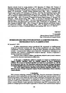
3. Implementations of GB-RNSA This section describes the implementation strategies of the proposed algorithm. The basic idea of the algorithm is described in Section 3.1. Sections 3.2, 3.3 and 3.4 are the detailed descriptions of the algorithm. The grid generation method is introduced in Section 3.2. Coverage calculation method of the non-self space is introduced in Section 3.3. And the filter method of candidate detectors is introduced in Section 3.4. Performance analysis of the algorithm is given in Section 3.5. Time complexity analysis of the algorithm is given in Section 3.6. 3.1. Basic Idea of the Algorithm. A real-valued negative selection algorithm based on grid GB-RNSA is proposed in this paper. The algorithm adopts variable-sized detectors and expected coverage of non-self space for detectors as the termination condition for detectors’ generation. The algorithm analyzes distributions of the self set in the real space and regards [0, 1]𝑛 space as the biggest grid. Then, through divisions step-by-step until reaching the minimum diameter of the grid and adopting 2𝑛 -tree to store grids, a finite number of subgrids are obtained, meanwhile self antigens are filled in corresponding sub grids. The randomly generated candidate detector only needs to match with selves who are in the grid where the detector is and in its neighbor grids instead of all selves, which reduces the time cost of distance calculations. When adding it into the mature detector set, the candidate detector will be matched with detectors within the grid where the detector is and neighbor grids, to judge whether the detector is in existing detectors’ coverage area or its covered space totally contains other detector. This filter operation decreases the redundant coverage between detectors and achieves that fewer detectors cover the non-self space as much as possible. The main idea of GB-RNSA is as shown in Algorithm 2. Iris dataset is one of the classic machine learning data sets published by the University of California Irvine [20], which are widely used in the fields of pattern recognition, data mining, anomaly detection, and so forth. We choose data records of category “setosa” in the dataset Iris as self antigens, choose “sepalL” and “sepalW” as antigen properties of first dimension and second dimension, and choose top 25 records of self antigens as the training set. Here, we use only two features of records, for that two-dimensional map is intuitive to illustrate the ideas, which does not affect
comparison results. Figure 1 illustrates the ideas of GB-RNSA and the classical negative selection algorithms RNSA and V-Detector. RNSA generates detectors with fixed radius. VDetector generates variable-sized detectors by dynamically determining the radius of detectors, through computing the nearest distance between the center of the candidate detector and self antigens. Detectors generated by the two algorithms need to conduct tolerance with all self antigens, which will lead to redundant coverage of non-self space between mature detectors with the increase of coverage rate. GB-RNSA first analyzes distributions of the self set in the space, and forms grids. Then, the randomly generated candidate detector only needs to perform tolerance with selves within the grid where the detector is and neighbor grids. Certain strategies are conducted for detectors which have passed tolerance, to avoid the duplication coverage and make sure that new detectors cover uncovered non-self space. 3.2. Grid Generation Method. In the process of grid generation, a top-down method is selected. First, the algorithm regards the 𝑛-dimensional [0, 1] space as the biggest grid. If there are selves in this grid, divide each dimension into two parts and get 2𝑛 sub grids. Then, continue to judge and divide each sub grid, until a grid does not contain any selves or the diameter of the grid reaches the minimum. Eventually, the grid structure of the space is obtained, and then the algorithm searches each grid to get neighbors in the structure. This process is shown in Algorithms 3 and 4. Definition 9 (minimum diameter of grids). 𝑟𝑔𝑠 = 4𝑟𝑠 + 4𝑟𝑑𝑠 , where 𝑟𝑠 is the self radius and 𝑟𝑑𝑠 is the smallest radius of detectors. Suppose that the diameter of a grid is less than 𝑟𝑔𝑠 , then divide this grid; the diameter of sub grids is less than 2𝑟𝑠 + 2𝑟𝑑𝑠 . If there are selves in the sub grid, it is probably impossible to generate detectors in the sub grid. So, set the minimum diameter of grids 4𝑟𝑠 + 4𝑟𝑑𝑠 . Definition 10 (neighbor grids). If two grids are adjacent at least in one dimension, these two grids are neighbors, which are called the basic neighbor grids. If selves of the neighbor grid are empty, add the basic neighbor grid of it in the same direction as the attached neighbor grid. The neighbors of a grid include the basic neighbor grids and the attached ones. The filling process of neighbor grids is shown in Algorithm 5.
4
Abstract and Applied Analysis
1
1
0.8
0.8
0.6
0.6
0.4
0.4
0.2
0.2
0
0 0
0.5 Self training set
1
0
1
1
0.8
0.8
0.6
0.6
0.4
0.4
0.2
0.2
0
0.5 RNSA
1
0.5
1
0 0
0.5 V-Detector
1
0
GB-RNSA
Figure 1: Comparison of RNSA, V-Detector, and GB-RNSA. (To reach the expected coverage 𝐶exp = 90%, three algorithms resp., need 561, 129, and 71 mature detectors, where the radius of self is 0.05, the radius of detector for RNSA is 0.05, and the smallest radius of detectors for V-Detector and GB-RNSA is 0.01).
𝐺𝐵-𝑅𝑁𝑆𝐴(𝑇𝑟𝑎𝑖𝑛, 𝐶exp , 𝐷) Input: the self training set 𝑇𝑟𝑎𝑖𝑛, expected coverage 𝐶exp Output: the detector set 𝐷 𝑁0 : sampling times in non-self space, 𝑁0 > max(5/𝐶exp , 5/(1 − 𝐶exp )) 𝑖: the number of non-self samples 𝑥: the number of non-self samples covered by detectors 𝐶𝐷: the set of candidate detectors 𝐶𝐷 = {𝑑 | 𝑑 =< 𝑦1 , 𝑦2 , . . . , 𝑦𝑛 , 𝑟𝑑 >, 𝑦𝑗 ∈ [0, 1], 1 ≤ 𝑗 ≤ 𝑛, 𝑟𝑑 ∈ [0, 1]} Step 1. Initialize the self training set 𝑇𝑟𝑎𝑖𝑛, 𝑖 = 0, 𝑥 = 0, 𝐶𝐷 = 0, 𝑁0 = 𝑐𝑒𝑖𝑙𝑖𝑛𝑔(max(5/𝐶exp , 5/(1 − 𝐶exp ))) Step 2. Call 𝐺𝑒𝑛𝑒𝑟𝑎𝑡𝑒𝐺𝑟𝑖𝑑(𝑇𝑟𝑎𝑖𝑛, 𝑇𝑟𝑒𝑒𝐺𝑟𝑖𝑑, 𝐿𝑖𝑛𝑒𝐺𝑟𝑖𝑑𝑠) to generate grid structure which contains selves, where 𝑇𝑟𝑒𝑒𝐺𝑟𝑖𝑑 is the 2𝑛 -tree storage of grids and 𝐿𝑖𝑛𝑒𝐺𝑟𝑖𝑑𝑠 is the line storage of grids; Step 3. Randomly generate a candidate detector 𝑑new . Call 𝐹𝑖𝑛𝑑𝐺𝑟𝑖𝑑(𝑑new , 𝑇𝑟𝑒𝑒𝐺𝑟𝑖𝑑, 𝑇𝑒𝑚𝑝𝐺𝑟𝑖𝑑) to find the grid 𝑇𝑒𝑚𝑝𝐺𝑟𝑖𝑑 where 𝑑new is; Step 4. Calculate the Euclidean distance between 𝑑new and all the selves in 𝑇𝑒𝑚𝑝𝐺𝑟𝑖𝑑 and its neighbor grids. If 𝑑new is identified by a self antigen, abandon it and execute Step 3; if not, increase 𝑖; Step 5. Calculate the Euclidean distance between 𝑑new and all the detectors in 𝑇𝑒𝑚𝑝𝐺𝑟𝑖𝑑 and its neighbor grids. If 𝑑new is not identified by any detector, add it into the candidate detector set 𝐶𝐷; if not, increase 𝑥, and judge whether it reaches the expected coverage 𝐶exp , if so, return 𝐷 and the algorithm ends; Step 6. Judge whether 𝑖 reaches sampling times 𝑁0 . If 𝑖 = 𝑁0 , call 𝐹𝑖𝑙𝑡𝑒𝑟(𝐶𝐷) to implement the screening process of candidate detectors, and put candidate detectors which passed this process into 𝐷, reset 𝑖, 𝑥, 𝐶𝐷; if not, return to Step 3. Algorithm 2: The algorithm of GB-RNSA.
Abstract and Applied Analysis
5
𝐺𝑒𝑛𝑒𝑟𝑎𝑡𝑒𝐺𝑟𝑖𝑑(𝑇𝑟𝑎𝑖𝑛, 𝑇𝑟𝑒𝑒𝐺𝑟𝑖𝑑, 𝐿𝑖𝑛𝑒𝐺𝑟𝑖𝑑𝑠) Input: the self training set 𝑇𝑟𝑎𝑖𝑛 Output: 𝑇𝑟𝑒𝑒𝐺𝑟𝑖𝑑 is the 2𝑛 -tree storage of grids, 𝐿𝑖𝑛𝑒𝐺𝑟𝑖𝑑𝑠 is the line storage of grids Step 1. Generate the grid of 𝑇𝑟𝑒𝑒𝐺𝑟𝑖𝑑 with diameter 1, and set properties of the gird, including lower sub grids, neighbor grids, contained selves, and contained detectors; Step 2. Call 𝐷𝑖V𝑖𝑑𝑒𝐺𝑟𝑖𝑑(𝑇𝑟𝑒𝑒𝐺𝑟𝑖𝑑, 𝐿𝑖𝑛𝑒𝐺𝑟𝑖𝑑𝑠)to divide grids; Step 3. Call 𝐹𝑖𝑙𝑙𝑁𝑒𝑖𝑔ℎ𝑏𝑜𝑢𝑟𝑠(𝐿𝑖𝑛𝑒𝐺𝑟𝑖𝑑𝑠) to find neighbors of each grid. Algorithm 3: The process of grid generation.
𝐷𝑖V𝑖𝑑𝑒𝐺𝑟𝑖𝑑(𝑔𝑟𝑖𝑑, 𝐿𝑖𝑛𝑒𝐺𝑟𝑖𝑑𝑠) Input: 𝑔𝑟𝑖𝑑 the grid to divide Output: 𝐿𝑖𝑛𝑒𝐺𝑟𝑖𝑑𝑠 the line storage of grids Step 1. If there are not any self or the diameter reaches 𝑟𝑔𝑠 of grid, don’t divide, add 𝑔𝑟𝑖𝑑 into 𝐿𝑖𝑛𝑒𝐺𝑟𝑖𝑑𝑠, and return; if not, execute Step 2; Step 2. Divide each dimension of 𝑔𝑟𝑖𝑑 into two parts, then get 2𝑛 sub grids, and map selves of 𝑔𝑟𝑖𝑑 into the sub grids; Step 3. For each sub grid, call 𝐷𝑖V𝑖𝑑𝑒𝐺𝑟𝑖𝑑(𝑔𝑟𝑖𝑑.𝑠𝑢𝑏, 𝐿𝑖𝑛𝑒𝐺𝑟𝑖𝑑𝑠). Algorithm 4: The process of 𝐷𝑖V𝑖𝑑𝑒𝐺𝑟𝑖𝑑.
𝐹𝑖𝑙𝑙𝑁𝑒𝑖𝑔ℎ𝑏𝑜𝑢𝑟𝑠(𝐿𝑖𝑛𝑒𝐺𝑟𝑖𝑑𝑠) Input: 𝐿𝑖𝑛𝑒𝐺𝑟𝑖𝑑𝑠 the line storage of grids Step 1. Obtain the basic neighbor grids for each grid in the structure 𝐿𝑖𝑛𝑒𝐺𝑟𝑖𝑑𝑠; Step 2. For each basic neighbor of every grid, if selves of this neighbor are empty, complement the neighbor of this neighbor in the same direction as an attached neighbor for the grid; Step 3. For each attached neighbor of every grid, if selves of this neighbor are empty, complement the neighbor of this neighbor in the same direction as an attached neighbor for the grid. Algorithm 5: The filling process of neighbor grids.
Figure 2 describes the dividing process of grids. The self training set is also selected from records of category “setosa” of the Iris data set. Select “sepalL” and “sepalW” as antigen properties of first dimension and second dimension. As shown in Figure 2, the two-dimensional space is divided into four sub grids in the first division, and then continue to divide sub grids whose selves are not empty, until the subs cannot be divided. Figure 3 is a schematic drawing of neighbor grids, and grids with slashes are the neighbors of grid [0, 0.5, 0.5, 1] which positions in the up-left of the space. 3.3. Coverage Calculation Method of the Nonself Space. The non-self space coverage 𝑃 is equal to the ratio of the volume 𝑉covered covered by detectors and the total volume 𝑉nonself of nonself space [12], as is shown in the following: 𝑑𝑥 ∫ 𝑉 𝑃 = covered = covered . 𝑉nonself ∫nonself 𝑑𝑥
(4)
Because there is redundant coverage between detectors, it is impossible to calculate (4) directly. In this paper, the probability estimation method is adopted to compute the detector coverage 𝑃. For detector set 𝐷, the probability of
sampling in the non-self space covered by detectors obeys the binomial distribution 𝑏(1, 𝑃) [13]. The probability of sampling 𝑚 times obeys the binomial distribution 𝑏(𝑚, 𝑃). Theorem 11. When the number of non-self specimens of continuous sampling 𝑖 ≤ 𝑁0 , if (𝑥/√𝑁0 𝑃(1 − 𝑃)) − √𝑁0 𝑃/(1 − 𝑃) > 𝑍𝛼 , the non-self space coverage of detectors reaches 𝑃. 𝑍𝛼 is 𝑎 percentile point of standard normal distribution, 𝑥 is the number of non-self specimens of continuous sampling covered by detectors, and 𝑁0 is the smallest positive integer which is greater than 5/𝑃 and 5/(1 − 𝑃). Proof. Random variable 𝑥 ∼ 𝐵(𝑖, 𝑃). Set 𝑧 = 𝑥 − 𝑁0 𝑃/ √𝑁0 𝑃(1 − 𝑃) = (𝑥/√𝑁0 𝑃(1 − 𝑃)) − √𝑁0 𝑃/(1 − 𝑃). We consider two cases. (1) If the number of non-self specimens of continuous sampling 𝑖 = 𝑁0 , known from De Moivre-Laplace theorem, when 𝑁0 > 5/𝑃 and 𝑁0 > 5/(1 − 𝑃), 𝑥 ∼ 𝐴𝑁(𝑁0 𝑃, 𝑁0 𝑃(1 − 𝑃)). That is, 𝑥 − 𝑁0 𝑃/ √𝑁0 𝑃(1 − 𝑃) ∼ 𝐴𝑁(0, 1), 𝑧 ∼ 𝐴𝑁(0, 1). Do assumptions that 𝐻0 : the non-self space coverage of detectors ≤ 𝑃; 𝐻1 : the non-self space coverage of detectors > 𝑃. Given significance level 𝑎,
6
Abstract and Applied Analysis 1
1
1
0.8
0.8
0.8
0.6
0.6
0.6
0.4
0.4
0.4
0.2
0.2
0.2
0
0 0
0.5
1
0 0
0.5
1
0
0.5
1
Figure 2: The process of grid division.
reaches the expected coverage 𝑃, and the sampling process stops. If not, increase 𝑖. When 𝑖 is up to 𝑁0 , put candidate detectors of CD into the detector set 𝐷 to change the nonself space coverage, and then set 𝑖 = 0, 𝑥 = 0 to restart a new round of sampling. With the continuous addition of candidate detectors, the size of the detector set 𝐷 is growing, and the non-self space coverage gradually increases.
1
0.8
0.6
0.4
0.2
0 0
0.5
1
Figure 3: The neighbor grids.
𝑃{𝑧 > 𝑍𝛼 } = 𝑎. Then, the rejection region 𝑊 = {(𝑧1 , 𝑧2 , . . . , 𝑧𝑛 ) : 𝑧 > 𝑍𝛼 }. So, when (𝑥/√𝑛𝑃(1 − 𝑃))− √𝑛𝑃/(1 − 𝑃) > 𝑍𝛼 , 𝑧 belongs to the rejection region, reject 𝐻0 , and accept 𝐻1 . That is, the non-self space coverage of detectors > 𝑃. (2) If the number of non-self specimens of continuous sampling 𝑖 < 𝑁0 , 𝑖 ⋅ 𝑃 is not too large, 𝑥 approximately obeys the Poisson distribution with 𝜆 equaling 𝑖 ⋅ 𝑃. Then 𝑃{𝑧 > 𝑍𝛼 } < 𝑎. When (𝑥/√𝑁0 𝑃(1 − 𝑃)) − √𝑁0 𝑃/(1 − 𝑃) > 𝑍𝛼 , the non-self space coverage of detectors > 𝑃. Proved.
From Theorem 11, in the process of detector generation, only the number of non-self specimens of continuous sampling 𝑖 and the number of non-self specimens covered by detectors 𝑥 need to be recorded. After sampling in the non-self space, determine whether the non-self specimen is covered by detectors of 𝐷. If not, generate a candidate detector with the position vector of this non-self specimen, and then add it into the candidate detector set CD. If so, compute whether (𝑥/√𝑁0 𝑃(1 − 𝑃)) − √𝑁0 𝑃/(1 − 𝑃) is larger than 𝑍𝛼 . If it is larger than 𝑍𝛼 , the non-self space coverage
3.4. Filter Method of Candidate Detectors. When the number of sampling times in the non-self space reaches 𝑁0 , detectors of candidate detector set will be added into the detector set 𝐷. At this time, not all candidate detectors will join 𝐷, and the filtering operation will be performed for these detectors. The filtering operation consists of two parts. The first part is to reduce the redundant coverage between candidate detectors. First, sort detectors in the candidate detector set in a descending order by the detector radius, and then judge whether the candidate detectors in the back of the sequence have been covered by the front ones. If so, this sampling of the non-self space is invalid, and the candidate detector generated from the position vector of this sampling should be deleted. There is no complete coverage between candidate detectors which have survived the first filtering operation. The second part is to decrease the redundant coverage between mature detectors and candidate ones. The candidate detector will be matched with detectors within the grid where the detector is and neighbor grids when adding it into the detector set 𝐷, to judge whether it totally covers some mature detector. If so, the mature detector is redundant and should be removed. The filtering operations ensure that every mature detector will cover the uncovered non-self space. The filtering process of candidate detectors is shown in Algorithm 6. 3.5. Performance Analysis. This section analyzes the performance of the algorithm from the probability theory. Assuming that the number of all the samples in the problem space is 𝑁𝐴𝑔 , the number of antigens in the self set is 𝑁𝑆𝑒𝑙𝑓 , the number of antigens in the training set is 𝑁𝑠 , and the number of detectors is 𝑁𝑑 . The matching probability between a detector and an antigen is 𝑃 , which is associated with
Abstract and Applied Analysis
7
𝐹𝑖𝑙𝑡𝑒𝑟(𝐶𝐷) Input: the candidate detector set 𝐶𝐷 Step 1. Sort CD in a descending order by the detector radius; Step 2. Make sure that centers of detectors in the back of the sequence do not fall into the covered area of front detectors. That is to say, 𝑑𝑖𝑠(𝑑𝑖 , 𝑑𝑗 ) > 𝑟𝑑𝑖 , where 1