A Recurrent Neural Network that Learns to Count - Computational

Connection Science, Vol. 11, No. 1, 1999, 5± 40

A Recurrent Neural Network that Learns to Count

PAUL RODRIGUEZ, JANET W ILES & JEFFREY L. ELMAN

Parallel distributed processing (PDP) architectures demonstrate a potentially radical alternative to the traditional theories of language processing that are based on serial computational models. However, learning complex structural relationships in temporal data presents a serious challenge to PDP systems. For example, automata theory dictates that processing strings from a context-free language (CFL) requires a stack or counter memory device. While some PDP models have been hand-crafted to emulate such a device, it is not clear how a neural network might develop such a device when learning a CFL. This research employs standard backpropagation training techniques for a recurrent neural network (RNN) in the task of learning to predict the next character in a simple deterministic CFL (DCFL). We show that an RNN can learn to recognize the structure of a simple DCFL. We use dynamical systems theory to identify how network states re¯ ect that structure by building counters in phase space. The work is an empirical investigation which is complementary to theoretical analyses of network capabilities, yet original in its speci® c con® guration of dynamics involved. The application of dynamical systems theory helps us relate the simulation results to theoretical results, and the learning task enables us to highlight some issues for understanding dynamical systems that process language with counters. KEYWORDS:

Recurrent neural network, dynamical systems, context-free languages.

1. Introduction It is well established that sentences of natural language are more than just a linear arrangement of words. Sentences also contain complex structural relationships between words that are often characterized syntactically, such as phrase structures, relative clauses and subject± verb agreement. Representing and processing such structure presents a critical challenge to mechanisms of natural language processing (NLP) as a gauge of both their theoretical capabilities and their potential to provide a psychological account of natural language parsing. A traditional view of NLP is based on mechanisms of ® nite automata, in which discrete states and transitions between states specify the temporal processing of the system. On the other hand, parallel distributed processing (PDP) architectures demonstrate a potentially radical alternative to the traditional theories of language processing. In particular, a recurrent neural network (RNN) is a PDP model that implements temporal processing through feedback connections. Contrary to P. Rodriguez and J. L. Elman, Department of Cognitive Science, U niversity of California at San Diego, La Jolla, CA 92093-051 5, USA. E-mail: [email protected]. Janet W iles, Departments of Computer Science and Psychology, U niversity of Queensland, Queensland 4072, Australia. 0954-0091 /99/010005-36 $9.00

€ 1999 Carfax Publishing Ltd

6

P. Rodriguez et al.

discrete automata, an RNN has continuous-valued states that are functions of previous states. In this sense, an RNN is a dynamical system; and an RNN that processes language is an example of a dynamical recognizer (Pollack, 1991). Research that investigates RNNs as language processors has been based on both empirical simulations and theoretical analysis of dynamical systems. Empirical approaches have shown interesting behavior of RNNs that re¯ ect some aspects of performance and some aspects of theoretical capabilities in processing natural and arti® cial languages (e.g. Elman, 1991; Giles et al., 1992; Servan-Shrieber et al., 1988). Theoretical approaches have been guided by traditional automata theories and have formally shown that a dynamical system can be constructed as an RNN to simulate universal Turing machines (Pollack, 1987b; Siegelmann, 1993). However, many questions remain to be investigated with respect to the kind of computational hierarchy embodied in dynamical systems, and how they are implemented or learned in RNNs. The work reported here is an empirical investigation which is complementary to theoretical analyses, yet original in its speci® c con® guration of dynamics involved. Our results demonstrate how an RNN can implement the kind of solutions used in the formal dynamical recognizer analysis. Speci® cally, we show that an RNN that performs a prediction task can learn to process a simple deterministic contextfree language (DCFL), a n b n , in a way that generalizes to longer strings by developing up /down counters in separate regions of phase space. The solution is novel because it uses a saddle point and the trajectories oscillate around the ® xed points. The analysis demonstrates an application of dynamical systems theory to the study of RNNs and helps identify properties of the trajectories that may be especially relevant to learnability and representation for connectionist models of language processing. 2. Background Automata theory states that a regular language (R L) can be processed by a ® nite state machine (FSM). However, a language with center-embedding is at least a context-free language (CFL), for which at least a push-down automaton (PDA) is required (Hopcroft & Ullman, 1979). Importantly, a PDA is an FSM with an additional resource of a memory-like device that is a stack or counter to keep track of the embeddings. Learning complex structural relationships in temporal data, such as CFLs, presents a serious challenge to systems which do not have a distinct memory device. An RNN can be hand-crafted to emulate such a device, but it is not clear how a network might develop such a device when learning a CFL. Empirical investigations using RNNs with simple arti® cial grammars have shown that an RNN can learn to recognize strings from an R L (Giles & Omlin, 1993; Giles et al., 1992; Servan-Shrieber et al., 1988; Smith & Zipser, 1989; Waltrous & Kuhn, 1992). It has also been shown that an RNN can implement FSM computations, such as push± pop transitions for a PDA (Sun et al., 1990) and the read / write /shift transitions for a Turing machine (Cottrell & Tsung, 1993; W illiams & Zipser, 1989). In fact, analysis has shown that an RNN can use regions of hidden unit space and transitions between regions to mimic states and transitions between states in an FSM (Casey, 1996; Giles et al., 1992). Owing to limited computer precision, an RNN can only represent a ® nite number of regions of space, thereby never achieving more than the capability of an FSM. Consequently, the argument could be made that any attempt to learn a CFL by an RNN simulation will only

An RNN that Lear ns to Count

7

result in an FSM -like approximation with limited or no generalizationÐ but we shall show otherwise. There has been relatively less work using RNNs with arti® cial CFLs. Work with the recursive auto-associative memory model (R AAM) has been successful at showing that an RNN can learn to perform push and pop functions that encode and decode tree structures, analogous to a stack, thereby exhibiting compositional structure (Blank et al., 1992; Kwasny & Kalman, 1995; Pollack, 1988). Pollack (1988, 1990) showed that a R AAM network can learn tree structures for simple context-free grammars, with some systematic generalization to unseen cases. Kwasny and Kalman (1995) trained a R AAM network with a simple DCFL , a balanced parenthesis language, and it was able to generalize to at least one more level of embedding, from four levels to ® ve. However, in these cases it was not shown that the R AAM can learn to generalize to much longer input strings or represent an unlimited number of embeddings. In contrast to the R AAM model, several researchers have used a simple recurrent network (SRN) in a prediction task to model sentence processing capabilities of RNNs. For example, Elman reports an RNN that can learn up to three levels of center-embeddings (Elman, 1991). Stolcke reports an RNN that can learn up to two levels of center-embeddings, and up to ® ve levels for tailrecursion (Stolcke, 1990). Other work has shown that an RNN can process temporal semantic cues within sentences and thereby re¯ ect semantic constraints and associations (St. John, 1990).1 It has also been shown that an RNN can handle more levels of embedding if there are additional semantic constraints (Weckerley & Elman, 1992), which suggests that the RNN is a mechanism that re¯ ects performance. However, in all these latter studies it may be the case that the RNN is performing the functional equivalent of an FSM. In other words, the RNN may not appropriately re¯ ect the syntactic structure of complex sentences as does a PDA. Pollack (1987a) showed that a second-order RNN can learn to develop an up / down counter to accept/reject strings from a balanced parenthesis language, but he did not show that it generalized to longer strings. Recently, it was shown that a ® rst-order RNN can perform prediction of strings from a DCFL, but the network could not generalize properly (Batali, 1994; Christiansen & Chater, 1994). In these cases, although the network clearly developed a counting function, it was not clear whether the network could learn function and process strings longer than seen in training. Kolen (1994) points out that both the R AAM and SRN are examples of dynamical systems that fall under the general framework of iterated function systems, and with real-valued variables they are capable of representing in® nite state systems. Blair and Pollack (1997) and Pollack (1991) showed how an RNN that learns an R L can represent an in® nite state machine as one looks at higher resolution of phase space partitions, even though the RNN looks like an FSM at lower resolution. In this work, we give an example of how an RNN actually re¯ ects an in® nite state system for a simple DCFL a n b n . Our architecture is the same as an SRN and we use the prediction task, but we use backpropagation through time training. As with earlier work, the network develops up /down counters, but in order to keep predictions linearly separable, the counters are in diþ erent regions of phase space. This work is distinct from other proposed modeling of CFLs by R AAMs, in that we are not directly attempting to represent constituent structures. Ultimately, we are more directly concerned with using a prediction task as a model

8

P. Rodriguez et al.

of performance, hence our analysis will show the nature of a solution that an RNN develops in this context. In the rest of the paper, we describe the RNN simulation experiment, present some concepts from dynamical systems theory, and apply the concepts to the analysis of the RNN simulations. We focus the analysis on two network results for comparison and then, later, discuss two further experiments: one with another simple DCFL (a balanced parenthesis language) and one that explores learning issues with more hidden units. We also describe how the RNN dynamics represent a solution that can process extremely long strings under ideal conditions. 3. RNN Simulation Experiment 3.1. Issues In this experiment we are concerned with the following two questions: (1) Can an RNN learn to process a simple DCFL with a prediction task? (2) What are the states and resources employed by the RNN? The ® rst question demands that an RNN learn to process a simple DCFL so that it generalizes beyond those input/output mappings presented in training. In other words, the performance of the RNN must somehow re¯ ect the underlying structure of the data. The second question demands a functional description of how the RNN re¯ ects the structure of the data. Ideally, one should ground the functional description of states and resources on a formal analysis of the RNN dynamics. First, we describe an RNN experiment to address the ® rst question; later, we describe some standard features of dynamical systems theor y as the method of analysis to address the second question. 3.2. Simulation Details 3.2.1. The input± output mapping task. The input stimuli consisted of strings from a very simple DCFL that uses two symbols, {a,b}, of the form a n b n . The input is presented one character at a time and the output of the network is trained to predict the next input in the sequence. Since the network outputs are not strictly binary, a correct prediction has a threshold value of 0.5. An example of the input± output mappings for network training is the following:

(note the transition at the last b should predict the ® rst a of the next string). Notice that when the network receives an a input, it will not be able to predict accurately the next symbol because the next symbol can be either another a or the ® rst b in the sequence. On the other hand, when the network receives a b input it should accurately predict the number of b symbols that match the number of a inputs already seen, and then also predict the end of the string (Batali, 1994). Correct processing to accept a string is de® ned as follows:

An RNN that Lear ns to Count

9

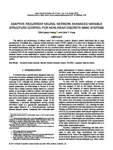
(1) for `b’ input Þ predict only `b’ symbols, except for (2); (2) on the last `b’ input Þ predict end of the string (or beginning of the next string). For a input there is not a clear criterion for what counts as correct predictions. It is relatively easy to hand-code a solution2 that always predicts b, except at the end of the string. However, we are much more interested in what the network can learn on its own. We might also add the condition that for an a input the network predict only an a output, but it will be seen that `good’ networks do this anyway to minimize error. Since the network does not explicitly accept/reject strings, as is typical in formal automata theory, our use of the prediction task raises an issue regarding the formal capabilities of the network. However, if the network makes all the right predictions possible, especially at the end of a string, then performing the prediction task subsumes the accept task. In our case, the network will always be presented with valid substrings so that the possibility of rejection will not explicitly arise. The restriction to legal strings does not invalidate the instructiveness of the RNN simulation results since there may be simple methods to include reject capabilities. For example, Das et al. (1992) trained an RNN to activate an explicit reject node for invalid strings. One could also add an extra output layer such that more complicated decision functions would be available. Furthermore, there are several advantages in the prediction task, as pointed out by Elman (1991). For example, it requires minimal commitment to de® ning the role of an external teacher and, perhaps most importantly, it is psychologically motivated by the observation that humans use prediction and anticipation in language processing (Kutas & Hillyard, 1984; McClelland, 1987). 3.2.2. Training set. The training set was purposely skewed towards having more short strings than long strings. The main reason is that we did not want the network to settle into a solution for a*b*. Rather, we wanted the network learn to process both long strings and the end-of-string transition of b to a, which required some skew. Although we did not do a systematic search of training sets, we did ® nd solutions using diþ erent proportions of long and short strings. We present results that we felt had a nice contrast to demonstrate the network solution. The training set we used contained 390 strings, where for each string 1 < n < 11; in other words, there was a maximum total length of 22 (11 as followed by 11 bs). The strings were presented in random order for a total of 2652 characters in sequence. There were more short strings than long strings in the following proportions: 10 strings of n 5 1, six strings of n 5 2, four strings of n 5 3, three strings of n 5 4, one string each for n > 5. The test set consisted of one copy of each string where 1 < n < 11, plus strings with n > 11. A network was considered to have generalized if that network had properly learned the training set and produced correct outputs for strings of length n > 11, up to the ® rst string that failed, such that the longer the string processed, then the better the network had generalized. 3.2.3. Architecture. The architecture for the experiment was an RNN with two input units, two hidden units, two copy units (which provide recurrent connections from the hidden units), two output units and one bias unit (see Figure 1). The bias unit was always set to a value of 1. The input units were set to values of [1 0] for the `a’ input, and [0 1] for the `b’ input. In one time step each bias, input and

10

P. Rodr iguez et al.

Figure 1. A recurrent neural network with two input lines, two hidden nodes, two output nodes, and a bias input to hidden nodes and output nodes. In one time step activation values for hidden nodes and output nodes are calculated based on the input line and copy unit values. The recurrent connections are realized through copy units which save the hidden unit values at one time step and then inject those values at the next time step. copy unit values were presented to the network. In the same time step the hidden unit activation values and then output unit activation values were updated. The copy units were then updated with the hidden unit activation values in preparation for the next time step. The copy units were initialized to zero for the ® rst input presentation and were not reset for each string.

3.3. Training We used the `backpropagation through time’ (BPTT) training algorithm (Rumelhart et al., 1986) implemented in our local simulator. During training the network is unfolded in time and several hidden layer copies are maintained. Although we did not systematically vary the number of copies, we found solutions with as few as eight copies for training sets that had a maximum size of n 5 11. The results we analyze in detail used 12 copies of hidden units for training. After training, the network is `folded back up’ so that there is only one set of weights. The only parameters we varied during training were the initial random seed, the length of training and the learning rate. In no case did we use momentum. We present networks that were trained to the point where they could generalize best, which is

An RNN that Lear ns to Count

11

not necessarily the same point at which it achieves a lowest mean squared error (M SE) measure. We often found better results in the network performance by using smaller learning rate parameters for short periods of training, as detailed below.

3.4. Results Out of 50 trials we found eight networks that successfully learned the training set and generalized. W ith more hidden units we found solutions more often, but the task still required lots of training. However, since we are more interested in identifying the nature of a solution, we ® rst present in detail two cases of network results and then, later, after understanding the solution, we discuss overall learning tallies of networks under various conditions. Of the two networks we will discuss, one network resulted in an incomplete solution and the other produced a solution that successfully generalized. The former will be useful in understanding the conditions for generalization. Both cases use the same network architecture and the same training set, but have diþ erent sets of initial weights (e.g. diþ erent initial seeds). In each case the initial weights were randomly chosen to be greater than 2 0.3 and less than + 0.3. The ® rst network was trained for approximately 2 million sweeps,3 or about 294 000 strings, with a learning rate value of 0.01, and then trained for another 100 000 sweeps with a smaller learning rate value of 0.001, for a total of 2.1 million sweeps. The network only learned proper predictions for n < 8. We tried various combinations of sweeps and learning rate values but no other performed better with this particular initial set of weights, although many combinations performed as well. The second network was trained for approximately 1 million sweeps, or about 147 000 strings, with a learning rate value of 0.01, 100 000 sweeps with a learning rate value of 0.0001, and 20 000 sweeps with a learning rate value of 0.00001. Again, we did not ® nd any other combination of sweeps and learning rate values that performed better with this initial set of weights. The network learned proper predictions for n < 16, for a total string length of 32. The MSE for the sample training set was about 0.248 for the ® rst network, and about 0.303 for the second network.4 The ® rst network attempts to solve the problem in an intuitive way, although it fails. The second network found a solution that does generalize, although the solution is non-intuitive and requires a dynamical systems analysis to explicate. Consequently, before we present the results in detail, in the next section we introduce the concepts and formalisms of dynamical systems theory.

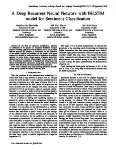
4. Method of Analysis 4.1. An RNN is a Dynamical System A discrete-time RNN can be characterized as a discrete-time dynamical system (e.g. Casey, 1996; Kolen, 1994; Pollack, 1991; Tino et al., 1995; Tsung & Cottrell, 1994). In each time step there is some vector of input values, some vector of copy unit values and a bias input which all feed a set of sigmoid activation functions that updates the vector of hidden unit values (see Figure 2). If the weight parameters are frozen (as they are after training) and the input values are held constant for several time steps,5 then the hidden unit activation values are the state variables in

12

P. Rodr iguez et al.

Figure 2. An RNN can be interpreted as a dynamical system. After training, the weights are frozen and each input condition is a constant for some number of iterations, until that input changes. Note that there is a diþ erent set of dynamics for each input condition and the phase space diagram is limited to the region [0,1] 3 [0,1] since the sigmoid activation function squashes all values to within that range.

a phase space diagram. In our simulations, the coordinate point of the phase space diagram is the pair {hidden unit 1, hidden unit 2} ({HU1,HU2}) and the vector `¯ ow’ ® eld6 gives a qualitative description of the change in activation values over time (e.g. the trajectory). Note that for each input there will be a diþ erent set of autonomous dynamics. Hence, for our experiment there will be one phase space diagram for the system of equations with a input (Fa system), and one phase space diagram for the system of equations with b input (F b system). Each output unit of an RNN is a function of the hidden unit activation values and therefore is not described as a state variable of a dynamical system. One could graph the output units in a three-dimensional coordinate system with {HU1,HU2} as the X,Y axis and the output unit as the Z axis. Instead, it will be more informative

An RNN that Lear ns to Count

13

to draw a contour plot for each output unit on the phase space trajectory diagrams. Since the output unit threshold of our task is 0.5, our ® gures have a one-line contour plot which partitions the phase space such that for all {HU1,HU2} values on one side of the line the output unit is > 0.5, and all values on the other side of the line the output unit is < 0.5. 4.2. Dynamical Systems Concepts In Appendix A we present formal de® nitions of concepts from dynamical systems theory. The formal concepts are most useful for understanding how the network may process unlimited length strings in principle. For the analysis below, we are mostly interested in the particular con® guration of attracting points, repelling points, and the trajectories realized by the hidden unit values for each input condition. Informally, if the system trajectory contracts towards a ® xed point, then that point is attracting; otherwise, that point is repelling. It is important in our case that a repelling point may be contracting in one direction and expanding in another direction, in which case that point is called a saddle point. In order to understand network performance we use the standard technique of linearization for analyzing behavior near a ® xed point. The technique produces a linear system for which the eigenvalues govern how the trajectories are contracting or expanding, as speci® ed in item (9) in the Appendix. In the analysis we show that a comparison of eigenvalues and associated eigenvectors provides criteria by which to evaluate network solutions. 5. Results 5.1. Overall Results As stated earlier, we present two cases of the RNN training results. Network 1 learned the training set only for n < 8; network 2 learned the training set completely and generalized to strings with n 5 12 to n 5 16. We present ® rst a graphical analysis of network performance using vector ¯ ow ® elds and trajectory plots. The graphical analysis will provide only a qualitative description of the network dynamics and some insights into the mathematical analysis that follows. 5.2. Network 1: Failure to Generalize The output units cut up the phase space evenly along a nearly vertical decision line, such that all {HU1,HU2} values to the left of the line predict a output, and all {HU1,HU2} values to the right predict b output. Most networks, independent of overall performance, divided the phase space evenly, although not necessarily vertically. The decision line will be shown on trajectory diagrams as a line in the diagram. Figure 3 shows the vector ¯ ow ® eld for the two input conditions. Note that the vectors are scaled from their true magnitude, but the relative vector size still re¯ ects relative change in {HU1,HU2}. Fa and F b represent the systems for the a input condition and b input condition, respectively. Note that Fa has an attracting point near (0,0.35), and F b has an attracting point near (0,1). The vector ¯ ow ® eld presents a graphical view of network dynamics when presenting strings from the a n b n language. Essentially, the hidden units will change values according to the Fa

14

P. Rodr iguez et al.

Figure 3. Network 1 vector ¯ ow ® elds for the dynamical system with a input condition (Fa ), or b input condition (F b ). There is one attracting point for Fa near (0,0.35), F b has one attracting point near (0,1). Each arrow is a scaled version of the actual change in the {HU1,HU2} coordinate point at the tail of the arrow. Each arrow direction indicates the direction of one trajectory step for that coordinate point. dynamics for the a input, and then change values according to the F b dynamics for the b input. These dynamics form the basis for network performance, as will be shown in the following ® gures. Figure 4 shows the trajectories for some short strings, n 5 2 and n 5 3.7 Each arrow represents one time step, hence one input. The tail of the arrow is the value of {HU1,HU2} before the time step and the head represents the updated value of {HU1,HU2} after applying the activation functions. Note that the initial value was

An RNN that Lear ns to Count

15

Figure 4. Network 1 trajectories for n 5 2 and n 5 3. The nearly vertical line represents the 0.5 threshold decision boundary; the left side indicates an a prediction at the output nodes and the right side indicates a b output prediction. Each arrow represents one time step, hence one input value. The tail is the previous hidden unit coordinate value; the head is the updated value. The initial starting point for the ® rst a is about {0.05,0.99}, the ® nal b input ends at about the same value. The trajectory crosses the dividing line on the last b input, which equates to predicting the start of the next string.

16

P. Rodr iguez et al.

chosen by allowing the network to run for one or two short strings. Importantly, for each string the last b input causes a change in {HU1,HU2} that crosses over to the left of the dividing line, hence the network properly predicts an a when the last b is input. Not surprisingly, the last {HU1,HU2} value is near the initial starting value. Figure 5 shows the trajectories for n 5 8 and n 5 9. Note that the trajectory steps are increasingly shorter near the Fa attracting ® xed point. Also, the ® rst b input causes a transition to a region of phase space where the trajectory can take

Figure 5. Network 1 trajectories for n 5 8 and n 5 9. For n 5 8, the trajectory crosses the dividing line on only the last arrow; but for n 5 9 the trajectory crosses the line on the eighth b input, which is one time step too early. For n > 9 the network had similar results of making predictions for the start of the next string too early.

An RNN that Lear ns to Count

17

smaller step sizes as well. However, for n 5 9 the network crosses the dividing line on the eighth b, showing that the step sizes are not properly matched. One important feature is that network 1 performed most of the processing of a input along the HU2 axis, and most of the processing for b input along the HU1 axis. In fact, Fa monotonically decreased in HU2, and F b monotonically decreased in HU1, which intuitively suggests that the network is `counting as’ and then `counting bs’ , with a transition from a to b that attempts to set up a proper b starting point.

5.3. Network 2: Successful Generalization Network 2 also has output values that divide the phase space along a nearly vertical line (but not all networks had vertical dividing lines). The ¯ ow ® elds in Figure 6 show that Fa has an attracting point near (0,0.85). F b appears to have an attracting point near (0.4,0.8), however, this turns out to be an artifact of the scaling of the vector ® eld. Figure 7 shows a smaller region with unscaled vectors in a 3 3 3 array. Notice that the top row and bottom row bounce over the middle, but the middle row vectors are shorter and they cross over the middle of the array, which suggests that there is actually a repelling ® xed point near the middle. Simple computer iteration determined that starting at (0.4,0.8), the F b system activation values oscillate and eventually settle into a periodic-2 ® xed point. The presence of a periodic-2 ® xed point also implies that the system had a period-doubling bifurcation that created a repelling ® xed point. Figure 8 shows the dynamics for F 2b (the composite of F b with itself ). One can now see that F 2b has two ® xed points, near (0,0.4) and near (1,1). As it turns out, the trajectories for Fa also oscillate as they converge on the attractor. Figure 9 shows the trajectories for short strings, n 5 2 and n 5 3. Again, the arrows represent one time step, hence one input. In Figure 10, n 5 4 and n 5 5, one can see that the trajectories are actually oscillating around both the attracting point and the repelling point. Figure 11, n 5 11 and n 5 16, con® rms that the oscillations match for longer strings. In other words, if the last a input ends up a little higher (or lower) than the attracting ® xed point, then the ® rst b input must transition to a coordinate point that is also higher (or lower8 ) than the repelling ® xed point near (0.4,0.8). Also, the small steps of Fa must be matched by small steps of F b . As the F b trajectory steps expand around the repelling point, the network will cross the dividing line on the last expanding step after taking the correct number of small steps. We refer to such complementary dynamics as coordinated trajectories.

5.4. Analysis Results In this section we develop a deeper analysis of the networks and establish some informal criteria that explain how a network is successful. The analysis employs the standard technique of linearization for each input condition as follows. Step 1. Find the ® xed points. For some systems one can ® nd ® xed points by analytically solving the set of equations that de® ne the system. However, one cannot analytically ® nd an exact ® xed point solution for an RNN with sigmoid activation functions. Fortunately, after one freezes the weights one can easily ® nd attracting points by computer iteration of the activation functions. A repelling point

18

P. Rodr iguez et al.

Figure 6. Network 2 vector ¯ ow ® elds for Fa and F b . There is one attracting point for Fa near (0,0.85). F b seems to have one attracting point near (0.4,0.8) but, due to the oscillation dynamics around a saddle point, the scaled vectors are misleading (see Figure 7). can be found by ® rst estimating its location and then using standard methods to ® nd roots of the system of equations. Step 2. Evaluate the partial derivative at the ® xed point. The partial derivative of the RNN with sigmoid functions for two hidden units is given by the following matrix: DF 5

[

w h1 ,h1 (1 2

f1 ) ( f1 ) w h1,h2 (1 2

f1 ) ( f1 )

w h2 ,h1 (1 2

f 2 ) ( f 2 ) w h2,h2 (1 2

f2 ) ( f2 )

]

An RNN that Lear ns to Count

19

Figure 7. A close-up of the network 2 vector ¯ ow ® eld for F b using unscaled vectors in a 3 3 3 array. The vectors actually jump over the middle region and are smaller in the middle region, which suggests that there is a repelling point there.

Figure 8. Network 2 vector ¯ ow ® eld for F b composite with F b (written as F 2b ). There is a periodic-2 ® xed point near (0,0.4) and near (1,1). The F 2b ¯ ow ® eld shows that there is a saddle point, not an attracting point, near (0.4,0.8).

20

P. Rodr iguez et al.

Figure 9. Network 2 trajectories for n 5 2 and n 5 3. The nearly vertical line represents the 0.5 threshold decision boundary; the left side indicates an a prediction at the output nodes and the right side indicates a b output prediction. Each arrow represents one time step, hence one input value. The trajectories oscillate around the ® xed points but still manage to cross the dividing line on the last b input.

where w i, j is the weight to the i th hidden unit from the j th hidden unit and each function f i is evaluated at the ® xed point value. Each element of the matrix is the partial derivative of f i with respect to x j , where i is the row and j is the column. Step 3. Use the linear system with the partial derivative as the matrix of coeý cients. The linear system is set up as: X 5 [DF] ´ X.

An RNN that Lear ns to Count

21

Figure 10. Network 2 trajectories for n 5 4 and n 5 5. Again, the trajectory crosses the dividing line on the last b input. Step 4. Find the eigenvalues and eigenvectors of the linear system to infer the behavior of the non-linear system near the ® xed point. Steps 1 ± 4 are a standard method for evaluating the stability (attracting or repelling) of ® xed points in non-linear systems. Although in our experiment we already knew about the stability of the ® xed points (graphically and via iteration), we used this technique to compare the trajectories for Fa and F b in the neighborhood around the ® xed points. Since the graphs show that the interesting dynamics occur near the attracting point for Fa and the repelling point for F b , we used these two points in the linearization method.9

22

P. Rodr iguez et al.

Figure 11. Network 2 trajectories for n 5 11 and n 5 16. The small trajectory steps seem to be matched near the Fa attracting point and the F b repelling point. The results in Table I summarize our ® ndings. For comparison we included two other cases of networks with the same architecture trained on the same task, although with diþ erent combinations of initial seed, training set and learning rate values. Network 3 has dynamics similar to network 1.1 0 Network 4 has dynamics similar to network 2, which was reported earlier by Wiles and Elman (1995). The table compares the largest eigenvalues (in positive or negative magnitude) of the Fa system with the largest eigenvalue of the F b system. These eigenvalues are associated with the eigenvectors that correspond to the axis of contraction under Fa , and the axis of expansion under F b . The contraction and expansion rates, which are given by the eigenvalues, indicate the change in hidden unit values from one

An RNN that Lear ns to Count

23

Table I. A comparison of largest eigenvalues at the attracting ® xed point of Fa and repelling ® xed point of F b ; the successful networks, 2 and 4, have eigenvalues that are inversely proportional to each other Network 1 2 3 4

M ax n learned 8 16 7 25 2

2

Fa 0.408 0.7095 0.242 0.637

1/Fa

2

2

Fb 0.832 1.455 1.29 1.536 2

2

2.45 1.409 4.136 1.57

time step to the next. In other words, the size of the trajectory step, as seen in the graphical analysis, is determined by the eigenvalues. If the eigenvalues are inversely proportional, then step sizes for a input will be matched by step sizes for b input. Based on the results in the table, one criterion for successful counting is to have the rate of contraction for Fa around the attracting point and the rate of expansion for F b around the repelling point inversely proportional to each other. This criterion helps explain how the network predicts the transition at the end of the string. However, it does not explain how the network dynamics are con® gured so that the transition from the last a to the ® rst b in an input sequence will put the network in a region of phase space where the step sizes match. In other words, how does the network functionally copy over the value of the a count? We analyzed this by looking at the smaller eigenvalue and related eigenvector at the repelling point of the F b system. The smaller eigenvalue has a value less than one (about 0.3), which means that the repelling ® xed point is a saddle point. Figure 12 replicates the vector ¯ ow ® eld F b and F 2b , but we have also drawn in lines in the direction of the eigenvectors, which intersect at the location of the saddle point. The line that crosses the HU2 axis near (0,0.85) is the stable eigenvector line; and the line that crosses the HU2 axis near (0,0.65) is the unstable eigenvector line. Values of {HU1,HU2} near the stable eigenvector are contracted in towards the saddle point before moving towards the periodic-2 ® xed point. Notice that the attracting ® xed point for the Fa dynamics (see Figure 6) nearly falls on the stable eigenvector line of the saddle point for the F b dynamics. In Figure 13 we show the coordinate points for several of the ® rst b input transitions after a n where n 5 2 . . . 6. The points of the a sequence are contracted so that they are nearly aligned with the unstable eigenvector. Notice that points that are near to / far from the Fa attracting point are translated by the ® rst b input to points that are near to /far from the F b saddle point. Hence, a second criterion for counting in diþ erent regions of phase space is to have the attracting point of Fa lie on the stable manifold1 1 of the saddle point for F b , with a small enough eigenvalue, so that the system can copy over the a count value to the unstable manifold of the saddle point. Finally, we should also require that the system return to a correct starting point, which in principle could be achieved with another input symbol, such as an end marker, that resets the system. In our case, a third criterion is to have the F b trajectory return to the starting point, or, equivalently, the starting point should be located at the end of the F b trajectory. For example, in network 4, all cases of a n b n start and end in a region roughly between (0.09,0.85), (0.15,0.98) and (0.24,0.88). On the other hand, in network 2 the string a 1b 1 was solved separately since it could not use the same initial starting point as for a n b n, when n > 1. The start /end point

24

P. Rodr iguez et al.

Figure 12. Network 2 eigenvector lines, for F b saddle point, drawn on the vector ¯ ow ® eld for F b and F 2b . The eigenvector lines intersect at the saddle point. The F b diagram does not show the oscillatory dynamics because the arrows are scaled to one-tenth of the actual size. The arrows around the saddle point actually represent trajectories that `hop’ over the saddle point. However, it does show that arrows near the eigenvectors move in a direction along the eigenvectors. The F 2b diagram shows that trajectories along the stable eigenvector will move towards the saddle point ® rst and then towards one of the attracting points. Importantly, the stable eigenvector line crosses the HU2 axis near (0,0.85), which is near the attracting point for Fa , which accounts for how the ® rst b input condition places the {HU1,HU2} values close to the saddle point, thereby allowing the system to process the b input in a diþ erent region of phase space.

An RNN that Lear ns to Count

25

Figure 13. The transition of the ® rst b input after sequences of a input. Note that the b input aligns the points along the unstable eigenvector such that points near to /far from the Fa attracting ® xed point are translated to points near to /far from the stable eigenvector. for a n b n is near (0.15,0.65), but a correct starting point for a 1b 1 is near (0.05,0.5). However, a 1 b 1 terminates close enough to the good starting point so that a sequence of strings that start with a 1 b 1 will be processed correctly. Among the best networks, networks 2 and 4 nearly satisfy all three criteria. For the other networks, network 3 does not satisfy the ® rst criterion but otherwise did satisfy the second and third, and network 1 does not satisfy either the ® rst or second. The best networks are imperfect counters and the other networks are bad counters. In summary, the criteria describe suý cient conditions for an RNN to achieve coordinated trajectories that have the functional capability to process the a n b n language.

6. Balanced Parenthesis Language A more complicated DCFL, but still relatively simple, is the balanced parenthesis language.12 A string in this language consists of some number of as and the same number of bs, but a b can be placed anywhere such that it matches some previous a. In other words, a ba can be embedded anywhere in the string after the ® rst a (e.g. S ® ab ½ aXb; X ® ab ½ ba ½ aX*b). A network trained to predict the next input can only correctly predict the end of the string. Intuitively, the network must maintain the coordination of trajectories such that for any interweaving sequence of as and bs the system will still be able to predict the beginning of the next string when it gets the last b input. For example, in the string aababb the hidden unit values should be the same after aa as they are after aaba. In other words, any ba

26

P. Rodr iguez et al.

subsequence must return the system to a state on the same trajectory as the string without that subsequence. Since this prediction task is also a counting task, we asked if our network can process balanced parenthesis strings. Further testing of network 2 with strings from the balanced parenthesis language con® rms that coordinated trajectories can process the language. Figure 14 shows that network 2 will correctly predict the transition at the end of strings such as aabaabbb and aabaabaabbbb. In fact, the network also worked with longer strings,

Figure 14. Network 2 trajectories for strings from balanced parenthesis language. The only prediction possible for the network is to predict the start of the next string by crossing the dividing line on the last b input. Even though the network was not trained on such strings it does cross the dividing line properly on the last b for the input strings aabaabbb (total length 5 8) and aabaabaabbbb (total length 5 12).

An RNN that Lear ns to Count

27

Figure 15. Network 2 trajectory for balanced parenthesis string of aaaabaaaabbbaaabbbbaaaaaabbbbbbbbb (total length 5 34). Again, on the last b input the network crosses the dividing line.

as shown in Figure 15. This result is striking because the network was never trained on any string with a ba subsequence. Other tests showed that the network did not correctly process all strings of total length < 32 (e.g. 16 as and 16 bs). One reason seems to be that when it processed some strings it could not always return to a proper initial starting value, which inhibited processing of following strings (e.g. compare Figure 15 with Figures 9 ± 11). Nonetheless, the positive results suggest that network 2 dynamics reveal how to generalize to the balanced parenthesis language. In contrast, however, network 4 could process almost no such strings. An extension of the previous linearization analysis shows that only for network 2 does the F b saddle point fall near the second stable eigenvector (corresponding to the smaller eigenvalue) of the Fa attracting ® xed point (compare Figure 16 with Figure 12). The latter con® guration does not occur in network 4 (see Figures 17 and 18). In other words, for ba subsequences the network 2 dynamics can maintain coordinated trajectories by contracting the hidden unit values back on to the dominant contracting axis of Fa , which is where the system was processing the previous a input. This suggests that an additional criterion for an RNN that processes the balanced parenthesis language is to have the saddle point for F b lie on the stable eigenvector for the smaller eigenvalue of the Fa attracting point so that the system can return to a previous state of the a count.

7. Learning In this section we present some empirical results on learning with diþ erent training sets and more hidden units. Not surprisingly, the maximum length of network generalization is very sensitive to small changes in weight parameters. Tonkes

28

P. Rodr iguez et al.

Figure 16. Network 2 network vector ¯ ow ® eld for Fa with eigenvector lines at the attracting point drawn in. The eigenvector associated with the dominant eigenvalue is nearly vertical along the HU2 dimension, and the other line is nearly horizontal. Note that the saddle point of F b , approximately (0.4,0.8), lies near the eigenvector associated with the smaller, non-dominant eigenvalue. This corresponds to the ability of the network to handle ba subsequences of strings from the balanced parenthesis language.

Figure 17. Network 4 network vector ¯ ow ® eld for Fa with eigenvector lines at the attracting point drawn in. The eigenvector associated with the dominant eigenvalue is nearly vertical along the HU2 dimension.

An RNN that Lear ns to Count

29

Figure 18. Network 4 network vector ¯ ow ® eld for F 2b with eigenvector lines at the saddle point (near 0.6,0.85) drawn in. Similar to network 2, there is a period-2 ® xed point near {0.15,0.85} and {0.95,0.95}. Note that the saddle point does not fall near the eigenvector line for the smaller, non-dominant eigenvalue of Fa (see Figure 16), which indicates why the network cannot handle ba subsequences of the balanced parenthesis problem.

(1998), for example, has repeated our experiment and shown how the network cycles through periods of ® nding and losing good solutions during training. Also, the length of strings used in training had some interesting eþ ects. We found that no network developed oscillation dynamics around the ® xed points when the maximum length string in the training set was n 5 6 (total length 5 12), whereas some networks did for n 5 7. One reason may be that with a training set of shorter strings the network learns that a 6 is always followed by a b, whereas a 1 . . . a 5 are not. Therefore, the b output unit decision line will intersect the a input trajectory between a 5 and a 6 , which in turn inhibits trajectories that oscillate and converge around an attractor. Learning to process the a n b n language by our de® nition of correctness is not a trivial task for an RNN. We ran larger sets of simulations using the training set described in Section 3 and varying the number of hidden units. We found that with two hidden units eight out of 50 networks were successful,1 3 with three hidden units 18 out of 50 networks were successful, and with ® ve hidden units 24 out of 50 were successful.1 4 These admittedly rough statistics suggest that learning to process the language does require much training, but certainly is not rare. All of the successful networks developed oscillation dynamics around the ® xed points. We speculate that training a network that oscillates around the ® xed points may be related to phase space learning, as investigated by Tsung (1994). In that work Tsung demonstrated that RNN training is improved by providing input vectors that specify how nearby orbits should converge to an attractor. In our case, perhaps, oscillation dynamics perform better because the hidden unit activation

30

P. Rodr iguez et al.

values visit regions of phase space that surround the ® xed points, thereby enabling error signals that better tune the parameters. In contrast, monotonic dynamics only contract to (expand from) an attracting (repelling) point from one side such that the system does not receive error signals around the ® xed points. For example, in the network 3 monotonic solution, the F b saddle point results in two attracting points: one is near the starting point in the predict a region, and the other is in the predict b region. Often, during training, the network would incorrectly process long strings by transitioning into the wrong attractor region on the ® rst b input. We also investigated in detail the network solutions with more hidden units. We found that with more hidden units the dynamics are similar to that found in network 2, although in some cases the network would generalize better (e.g. up to n 5 21). Interestingly, in one network with ® ve hidden units the dynamics were similar to network 2 but with one novel diþ erenceÐ the dynamics were oscillating with periodicity of 5 and the F b system settled into a periodic-5 ® xed point. Although the dominant eigenvalues were not as closely inversely proportional as network 2, the network generalized just as far, up to n 5 16. One reason for the equivalent performance may be that the higher periodicity allowed the trajectory to `take up’ more regions of phase space and avoid expanding across the hyperplane that divides the a and b predictions too early. For example, on a test of n 5 17 the network with ® ve hidden units erred by making a prediction ® ve time steps too early on the twelfth b input. On the other hand, due to better matched eigenvalues, on a test of n 5 17 network 2 did not make a prediction error until the ® fteenth b, only two time steps too early. In addition, the network dynamics with ® ve hidden units became more distributed among hidden units, which con® rms that counting can be distributed among dimensions and that merely looking at individual hidden unit values may be misleading.

8. Finding the Lim it In this section we argue that the coordinated trajectory dynamics clearly represent a solution that could process the a n b n language for strings of unlimited length given unlimited precision. The argument is based on the dynamic properties of the linearized systems derived in the analysis (Section 5) for network 2. We construct a piecewise linear system that can work for strings of length n ® ` . Our construction is an example of the counting solutions in analog computation theory (e.g. Moore, 1996; Pollack, 1987b; Siegelmann, 1993), except that our system can have output predictions that are linearly separable. We then relate this to the non-linear system of an RNN and explore how well an RNN does in practice. Informally, the simple DCFL a n b n can be processed in a dynamical system by stipulating the piecewise linear function,

f (net) 5

{

1

net >

net

0 < net < 1

0

net 0, n > 0, is deterministic because of the change of symbols from w to w r at the middle. One way to process this language is to have an embedded counter for a n b n that keeps track of how many x inputs preceded the as in order to count the ys. We have results showing that an RNN can learn the task with some generalization such that an idealized version of the network dynamics re¯ ects a counting solution (Rodriguez & W iles, 1998). However, preliminary tests show that a palindrome

An RNN that Lear ns to Count

35

that has all possible sequences, e.g. w 5 (x or a)*, is a much harder problem. Although one can hand-code a piecewise linear solution easily enough, the network would have to learn to maintain information about all combinations, which would entail a fractal solution. 11. Conclusion Although the theoretical framework of discrete automata has established a hierarchy of complexity of formal languages and computation, the exact relationship of formal language computation to human language performance has not been fully established. One alternative is to develop an account based on processing with continuous-valued states, such as in dynamical systems. A proper approach seeks convergence of psycholinguistic data, empirical studies with RNNs, and theoretical analysis of dynamical recognizers to understand dynamical systems as a mechanism that may capture the complexity and hierarchies of natural language. Our work reported here helps draw together the study of RNNs using formal grammars, known classes of computability, learning and dynamical systems theory. The work adds a building block to the connectionist framework by showing that an RNN in a prediction task has the potential to go beyond a FSM . Rather, it can organize its resources to process dependencies in temporal data, such as strings from a DCFL, by coordinating the trajectories in phase space instead of adding an external stack /counter mechanism. Therefore, an RNN may not adhere to the same kind of resource diþ erences and computational metaphor embodied by traditional language-processing models based on discrete automata. Instead, an RNN may have similar capabilities without the same mechanistic discontinuities. Acknowledgements We bene® ted from helpful feedback from John Batali, Michael Casey, Gary Cottrell, Paul Mineiro, David Zipser, Mark St. John and three anonymous reviewers. This work was supported in part by the following grants: UCSD Department of Cognitive Science NSF Training Grant SBR-9256834, UCSD Center for Research in Language PHS5 T32 DC00041, and a McDonnell-Pew Center for Cognitive Neuroscience Visiting Scientist Award. Notes 1. There have been other works showing that feed-forward networks are capable of performing semantic processes, such as assigning thematic role information (M cClelland & Kawamoto, 1986; M iikkulainen, 1992). However, these do not show how a network can process temporal data. 2. An example is to use one hidden unit to count up and down. H owever, we found that no networks learned the prediction task with one hidden unit. 3. Each sweep is de® ned to be one presentation of an input pattern w ith the corresponding set of weight adjustments through error correction. 4. Some of the error in both cases is due to the fact that the network cannot predict the ® rst `b’ input. The case 1 network seemed to have a lower error since it often made predictions close to 1, even though it would not always correctly predict the end of string transition. W ith 1 m illion more sweeps the case 2 network M SE was even lower at 0.225, although it only generalized to n < 13. 5. W hen the parameters and input of a dynamical system are held constant it is often referred to as time-invariant and autonom ous. 6. In the case of a discrete system, each vector can be created by taking a sample of points in the coordinate system, then for each point apply the activation functions for one time step, and then

36

7.

8. 9. 10. 11.

12. 13. 14. 15.

16.

17.

P. Rodr iguez et al. use the new point as an arrow head (we thank M ike Casey for pointing this out to us). `Flow’ is a slight abuse of terminology, since it is normally used to refer to tangent vectors of continuous time systems. For the case n 5 1, the network can simply predict an a for both inputs in the ab sequence, which is not an interesting trajectory to display. Successful networks w ill sometimes require a few transient states (e.g. running the network with some short strings) in order to reach a good starting point to process n 5 1. M ore generally, higher or lower should be interpreted as one side or the other of the attracting point such that the system crossing the dividing line on the correct step. Network 1 did not actually have a repelling point, however, we used the point that had the smallest change in activation values, which still allows one to m ake a rough comparison of dynamics. Network 3 had dynamics that m onotonically increased for one hidden unit in Fa , then m onotonically decreased for the other hidden unit in F b , but in this case the F b dynamics have a saddle point. It is m ore correct to use the stable m anifold rather than stable eigenvector because, as we state in the Appendix, the non-linear system has a stable m anifold that is approximated by the stable eigenvector. In Section 8 we discuss this further. In fact, the language a n b n is a subset of the balanced parenthesis language. Success is de® ned here as no m ore than one error on the training set. We found that networks which m ade only one error typically had some generalization at some point in the training. Brad Tonkes ( personal communication) has found similar frequencies of learning results. Casey (1996) has shown a stronger statement that an RNN with ® nite number of hidden units cannot robustly process a CFL. We are not challenging this statement, but rather pointing out that these dynamics represent an idealized solution, not a physical realization of a solution (note that the same can be said of discrete automata). Since the case 1 network did not have a saddle point, it did not easily enable the same kind of m anipulation of ® xed points, w hich involves solving a system of equations based on the network weights while holding some weights and some coeý cients constant. In our case the location of the decision line is learned by the network; but see Kolen (1994) for a discussion of how the choice of decision function can aþ ect the interpretation of the computational capabilities of a system.

References Barton, G.E., Berwick, R.C. & Ristad, E.S. (1987) Computational Complexity and Natural Language. Cambridge, MA: M IT Press. Batali, J. (1994) Innate biases and critical periods: combining evolution and learning the acquisition of syntax. Arti® cial Life IV, pp. 160 ± 171. Cambridge, MA: MIT Press. Blair, A.D. & Pollack, J.B. (1997) Analysis of dynamical recognizers. Neural Computation, 9, 1127 ± 1142. Blank, D.S., M eeden, L.A. & M arshall, J.B. (1992) Exploring the symbolic /subsymbolic continuum: a case study of R AAM . In J. Dinsmore (E d.), Closing the G ap: Symbolism vs. Connectionism, pp. 113 ± 147. H illsdale, NJ: Lawrence Erlbaum Associates. Casey, M. (1996) The dynamics of discrete-time computation, with application to recurrent neural networks and ® nite state machine extraction. Neural Computation, 8, 1135 ± 1178. Christiansen, M .H . & Chater, N. (1994) Natural Language Recursion and Recurrent Neural Networks. T R 94-13 in Archive of Philosophy /Neuroscience/Psychology, Washington University. Cottrell, G.W. & Tsung, F.-S. (1993) Learning simple arithmetic procedures. Connection Science, 5, 37 ± 58. Das, S., G iles, C.L. & Sun, G.Z. (1992) Learning context-free grammars: capabilities and limitations of a recurrent neural network with an external m emory stack. Proceedings of the 14th A nnual Conference of the Cognitive Science Society, pp. 791 ± 796. Hillsdale, NJ: Lawrence Erlbaum Associates. Elman, J.L. (1991) Distributed representations, simple recurrent networks, and grammatical structure. M achine Lear ning, 7, 195 ± 225. G iles, C.L. & Om lin, C.W. (1993) Extraction, insertion and re® nement of symbolic rules in dynamically driven recurrent neural networks. Connection Science, 5, 307 ± 337. G iles, C.L., Sun, G.Z., Chen, H.H., Lee, Y.C . & Chen, D. (1992) Extracting and learning an unknown grammar with recurrent neural networks. In J.E. M oody, S.J. Hanson & R.P. Lippmann (E ds), A dvances in Information Processing 4, pp. 317 ± 323. San Mateo, CA: Morgan Kaufman. H opcroft, J.E. & U llman, J.D. (1979) Introduction to Automata Theory, Languages, and Computation. Addison-Wesley.

An RNN that Lear ns to Count

37

Kolen, J.F. (1994) Exploring the Computational Capabilities of Recurrent Neural Networks. PhD dissertation, T he Ohio State University. Kutas, M . & Hillyard, S.A. (1984) Brain potentials during reading re¯ ect word expectancy and semantic association. Nature, 307, 161 ± 163. Kwasny, S.C. & Kalman, B.L. (1995) Tail-recursive distributed representations and simple recurrent networks. Connection Science, 7, 61 ± 80. M artelli, M. (1992) Discrete Dynamical Systems and Chaos. Longman Scienti® c and Technical. M cClelland, J.L. (1987) The case for interactionism in language processing. In M. Coltheart (Ed.), A ttention and Performance XII: The Psychology of Reading. London: Erlbaum. M cClelland, J.L . & Kawamoto, A.H . (1986) Mechanism s of sentence processing: assigning roles to constituents. In D.E. Rumelhart & J.L . McClelland (Eds), Parallel Distributed Processing, Vol. 2. Cambridge, MA: M IT Press. M iikulainen, R. (1992) Script recognition with hierarchical feature maps. In N. Sharkey (Ed.), Connectionist Natural Language Processing, pp. 196 ± 214. Dordrecht: Kluwer Academic. M oore, C. (1996) Dynamical recognizers: real-time language recognition by analog computers. Santa Fe Institute Working Paper 96-05-023. Pollack, J.B. (1991) The induction of dynamical recognizers. Machine Lear ning, 7, 227 ± 252. Pollack, J.B. (1990) Recursive autoassociative m emories. Arti® cial Intelligence, 46, 77 ± 105. Pollack, J.B. (1988) Recursive autoassociative m emory: devising compositional distributed representations. Proceedings of the 10th A nnual Conference of the Cognitive Science Society, pp. 33 ± 38. Hillsdale, NJ: Lawrence Erlbaum Associates. Pollack, J.B. (1987a) Cascaded back propagation on dynamic connectionist networks. Proceedings of the 9th Annual Conference of the Cognitive Science Society, pp. 391 ± 404. Hillsdale, NJ: Lawrence Erlbaum Associates. Pollack, J.B. (1987b) On Connectionist Models of Language, PhD dissertation, Computer Science Department, U niversity of Illinois at U rbana-Champaign. Robinson, C. (1995) Dynamical Systems: Stability, Symbolic Dynamics, and Chaos. Boca Raton: CRC Press. Rodriguez, P. & W iles, J. (1998) A recurrent neural network can learn to implement symbol-sensitive counting. In M. Jordan, M. Kearns & S. Solla (Eds), Advances in Neural Information Processing Systems 10, pp. 87 ± 93. Cambridge, MA: M IT Press. Rumelhart, D.E., Hinton, G .E. & W illiams, R.J. (1986) Learning internal representations by error propagation. In D.E. Rumelhart & J.L. M cClelland (Eds), Parallel Distributed Processing, Vol. 2. Cambridge, MA: M IT Press. Servan-Schreiber, D., Cleermans, A. & M cClelland, J.L . (1988) Encoding Sequential Structure in Simple R ecur rent Networks. CMU T R CS-88-183, Carnegie M ellon U niversity. Siegelmann, H.T. (1993) Foundations of Recurrent Neural Networks. PhD dissertation, New Brunswick Rutgers, The State U niversity of New Jersey. Smith, A.W. & Zipser, D. (1989) Learning sequential structure with the real-time recurrent learning algorithm. International Journal of Neural Systems, 1, 125 ± 131. St. John, M. (1992) The story G estalt: a model of knowledge-intensive processes in text comprehension. Cognitive Science, 16, 271 ± 306. Stolcke, A. (1990) Lear ning Feature-based Semantics with Simple Recurrent Networks. TR-90-015, International Computer Science Institute, University of California at Berkeley. Sun, G.Z., Chen, H.H., G iles, C.L., Lee, Y.C. & Chen, D. (1990) Connectionist pushdown automata that learn context-free gramm ars. Proceedings of the International Joint Conference on Neural Networks, pp. I-577 ± 580. Washington, DC. Tino, P., Horne, B.G. & Giles, C.L. (1995) Finite State Machines and R ecur rent Neural Networks A utomata and Dynamical Systems A pproaches. TR-UM CP-CSD:CS-TR-3396, U niversity of Maryland, College Park. Tonkes, B. (1998) Recurrent networks are unstable in learning a simple context free language. 4th B iannual Australian Conference of Cognitive Science (in press). Tsung, F.-S. (1994) Modeling Dynamical Systems with Recurrent Neural Networks. PhD dissertation, Department of Computer Science, U niversity of California, San Diego. Tsung, F.-S. & Cottrell, G.W. (1994) Phase-space learning. In G. Tesauro, D. Touretzky & T. Leen (Eds), Advances in Neural Information Processing Systems 7. Cambridge, M A: MIT Press. Watrous, R.L . & Kuhn, G.M . (1992) Induction of ® nite-state automata using second order recurrent networks. In J.E. M oody, S.J. Hanson & R.P. Lippmann (E ds), Advances in Information Processing 4, pp. 309 ± 316. San Mateo, CA: M organ Kaufman. Weckerley, J. & Elman, J.L. (1992) A PDP approach to processing center-em bedded sentences.

38

P. Rodr iguez et al.

Proceedings of the 14th Annual Conference of the Cognitive Science Society, pp. 414 ± 419. H illsdale, NJ: Lawrence Erlbaum Associates. W iggins, S. (1990) Introduction to Applied Nonlinear Dynamical Systems and Chaos. New York: Springer. W iles, J. & Elman, J.L. (1995) Learning to count without a counter: a case study of dynamics and activation landscapes in recurrent neural networks. Proceedings of the 17th Annual Conference of the Cognitive Science Society, pp. 482 ± 487. Cambridge, M A: MIT Press. W illiams, R.J. & Zipser, D. (1989) Experimental analysis of the real-time recurrent learning algorithm . Connection Science, 1, 87 ± 111.

Appendix A: Dynamical Systems De® nitions In this section we present formal de® nitions of concepts from dynamical systems theory (see, for example, Martelli (1992), Tino et al. (1995), Robinson (1994) and W iggins (1990)). The formal concepts are useful when we discuss the principle of how the network may process in® nite-length strings. (1) A discrete-time dynamical system can be represented as the iteration of a diþ erentiable function: f: f

n

® f

n

,

e.g. x t + 1 5

f (x t ), t Î N, x Î f

n

where N denotes the set of natural numbers and f n denotes the n-dimensional space of real numbers. Note that the function f can be linear or non-linear, the diþ erence being that a linear function has the following property of superposition: f (cx + ky) 5 cf (x) + kf ( y), where c and k are scalar constants. (2) For each x Î f n , the iteration of f generates a sequence of distinct points which de® ne a trajectory of f. Given an initial state x 0 , the evolution of the system starting from x 0 is determined by the sequence of states: x0 , x 1 5

(3) (4) (5)

(6) (7)

f (x 0 ), x 2 5

f (x 1 ) 5

f 2(x 0 ), . . .

The sequence is called the trajectory of the system starting from x 0 . The sequence can also be de® ned as the set { f m (x 0 ) ½ m > 0}, where f m (x) is the composition of f with itself m times. A point x is called a ® xed point of f if f m(x ) 5 x , for all m Î N. A ® xed point x is called an attracting ® xed point of f if there exists a neighborhood around x , O(x ), such that lim m ® ` f m (x ) 5 x , for all x Î O(x ). A ® xed point x is called a repelling ® xed point of f if there exists a neighborhood around x , O(x ), such that lim m ® 2 ` f m(x ) 5 x , for all x Î O(x ). In other words, a repelling ® xed point is an attracting ® xed point in reverse sequence. A ® xed point x is called a periodic-2 ® xed point of f if f 2 (x ) 5 x . Note that a function may have a ® xed point of any period. A system of equations is a set of functions F 5 { f i : f n ® f n , i 5 1, 2, . . . }. For example, for a two-dimensional system, F 5 { f i , i 5 1,2}, x 1 ,t + 1 5 x 2 ,t + 1 5

f 1 (x 1,t , x 2 ,t ) f 1 (x 1,t , x 2 ,t )

(All the above de® nitions of ® xed points also hold for systems of equations.)

An RNN that Lear ns to Count

39

(8) For a linear system, F can be written as a matrix and the set of x i can be written as a vector X, such that X t + 1 5 F ´ X t . (9) An eigenvalue is a scalar k , and an eigenvector is a vector v, such that Fv 5 k v. For a linear system of n equations the eigenvalues give the rate of contraction or expansion and the eigenvectors give the axis along which the system contracts or expands. The eigenvalues, k i , i 5 1, 2, . . . , n, at the ® xed points determine the behavior of the system as follows: a) if k i < 1 and k i > 2 1, for all i, then the system is stable and contracting, and the ® xed point is an attracting ® xed point, b) if k i > 1 or k i < 2 1, for all i, then the system is expanding, and the ® xed point is a repelling ® xed point, c) if k j > 1 or k j < 2 1, for some integer(s) j, and if k i < 1 and k i > 2 1, for i 5 1, 2, . . . , j 2 1, j + 1, . . . , n, then the system is unstable and expanding in the direction of the eigenvector(s) that corresponds to k j , and the system is contracting in all other corresponding eigenvector directions. The ® xed point is also a repelling point speci® cally referred to as a saddle point. (The case of an eigenvalue 5 1 is de® ned to be non-hyperbolic and requires other methods to analyze the system around the ® xed point.) (10) For a non-linear system of equations, F, let DF 5 the partial derivative matrix ( Jacobian). There is a standard linearization technique for analyzing the behavior in the neighborhood of a ® xed point. The technique uses the DF matrix analyzed at the ® xed point, DF(x ), to produce a linear system, e.g. X 5 [DF(x )] ´ X. The eigenvalues of the linear system govern whether or not the non-linear system is contracting or expanding in the neighborhood of the ® xed point, just as for the linear system. (11) The non-linear system also contains invariant sets analogous to the linear system eigenvectors. These invariant sets are referred to as the stable manifold, and the unstable manifold. In the case of a saddle point there exists both a stable manifold and an unstable manifold. For a two-dimensional system each manifold is a curve tangent to the stable and unstable eigenvector at the saddle point, such that the following holds: (stable manifold) W S 5 {x ½ F(x) Î W S , and lim m ® ` F m (x) 5 x } (unstable manifold) W U 5 {x ½ F(x) Î W U , and lim m ® 2 ` F m (x) 5

x }

where x is the saddle point.

Appendix B: The Weights from Network 2 For completeness, we present the weights for network 2 discussed in the paper. Using an equation format where the weights are the matrix entries, H t is the state vector for hidden units at time t, It is the input vector which include the bias node (a 5 [1 1 0]Â , b 5 [1 0 1]Â ) and G is the sigmoid function: G(x) 5

1 1 + e2

x

40

P. Rodr iguez et al.

we have the equation: Ht 5

G

[

([ 2

2

3.4761645 4.4907968

3.080526

2

9.2054679

0.83122147

2

6.05627365

2

]

´ H t2

0.52505533

4.6773302

2.6301704

1.9219846

]

1

´ It

+

)

For the output unit vector, Y, the equation is: Yt 5

G

([ 2

1.4940302 1.4957459

2

5.2289746 5.22906011

2

0.58472942 0.58668607

]

´ H ²t

)

where H ² is the hidden unit vector augmented with the bias node as the ® rst entry.