Meter as Mechanism: A Neural Network that Learns ... - CiteSeerX

Meter as Mechanism: A Neural Network that Learns Metrical Patterns Michael Gasser, Douglas Eck and Robert Port

Cognitive Science Program Indiana University

Abstract

One kind of prosodic structure that apparently underlies both music and some examples of speech production is meter. Yet detailed measurements of the timing of both music and speech show that the nested periodicities that de ne metrical structure can be quite noisy in time. What kind of system could produce or perceive such variable metrical timing patterns? And what would it take to be able to store and reproduce particular metrical patterns from long-term memory? We have developed a network of coupled oscillators that both produces and perceives patterns of pulses that conform to particular meters. In addition, beginning with an initial state with no biases, it can learn to prefer the particular meter that it has been previously exposed to.

Meter in Music and Speech Meter is an abstract structure in time based on the periodic recurrence of pulses, that is, on equal time intervals between distinct phase zeros. From this point of view, the simplest meter is a regular metronome pulse. But often there appear meters with two or three (or rarely even more) nested periodicities with integral frequency ratios. A hierarchy of such metrical structures is implied in standard Western musical notation, where dierent levels of the metrical hierarchy are indicated by kinds of notes (quarter notes, half notes, etc.) and by the bars separating measures with an equal number of beats. For example, in a basic waltz-time meter, there are individual beats, all with the same spacing, grouped into sets of three, with every third one receiving a stronger accent at its onset. In this meter there is a hierarchy consisting of both a faster periodic cycle (at the beat level) and a slower one (at the measure level) that is 1/3 as fast, with its onset (or zero phase angle) coinciding with the zero phase angle of every third beat. This essentially temporal view of meter contrasts with the traditional symbol-string theories (such as Hayes, 1981 for speech and Lerdahl and Jackendo, 1983 for music). Metrical systems, however they are de ned, seem to underlie most of what we call music. Indeed, an expanded version of European musical notation is found to be practical for transcribing most music from around the world. That is, most forms of music employ nested periodic temporal patterns (Titon, Fujie, & Locke, 1996). Musical notation has

METER AS MECHANISM

2

often been used to describe human speech as well (Jones, 1932; Martin, 1972) even though clear empirical evidence for the appropriateness of the notation is not often provided and has proven very dicult to obtain (Dauer, 1983; Lehiste, 1977). Nevertheless, recently new experimental techniques have been developed that encourage the production of speech that is clearly structured by meter (Cummins & Port, 1998; Large & Jones, in press; McAuley & Kidd, in press; Tajima & Port, 1999). An awkward diculty is that the traditional de nition of meter employs the notion of an integer. Data on both music and speech show that the perfect temporal ratios predicted by such a de nition are never observed in performance. In musical performance, various kinds of temporal deviations in the timing speci ed by musical notation are well-known. And this is not merely Gaussian noise in time, but frequently systematic deviations from integer-ratio time intervals. These \stylistic features" may also be observed for individual performers (Todd, 1985). As for speech, claims of simple isochronous intervals between, say, stressed syllables in English or mora onsets in Japanese, have been debunked many times (Dauer, 1983; Port, Dalby, & O'Dell, 1987). In fact, the deviations are so large (Dauer, 1983) that some have questioned whether meter in speech may not be entirely a perceptual illusion (Lehiste, 1977; van Santen, 1996) with no basis whatever in the raw phenomena of speech production. We will suggest that this point of view is correct, at least insofar as it serves to emphasize the role of the perceptual mechanism. Whether the pattern is \really" in the sound or not is a philosophical issue. The important theoretical issue is whether there can be a notion of meter that does not depend on perfect integer ratios of time. If the intervals are variable and \noisy" or if they are systematically perturbed, then is the notion of meter appropriate at all, even when listeners report that they hear the meter and can tap their foot to it? Our answer is to say that there is meter in these cases. But to understand this kind of meter we must look beyond the simplistic assumptions about perfect isochrony and explore the measurement mechanism in detail. It seems that, in the end, the closest one can get to a formal theory of meter will be a running system that actually recognizes or \locks in" to a range of patterns that is close to what human listeners recognize. The best solution to the theoretical problem, then, is to propose that meter be de ned by reference to a speci c mechanism { a system that recognizes or deals responsively with metrically structured stimulation. If we can design a mechanism which prefers the integer ratios of the standard de nition but is tolerant of variation, then we may have an initial account of the kind of meter that humans actually produce and perceive when doing speech and music. There has been recent progress in this direction with the development of adaptive oscillator models that adjust their frequency and phase to a sequence of input pulses (Large & Jones, in press; Large & Kolen, 1994; McAuley, 1995; McAuley & Kidd, in press). These models can recognize simple metrical patterns of pulses despite the presence of noise on interpulse intervals. This is a major step forward, but still they are not able either (1) to learn to prefer one kind of meter over another based on experience or (2) to learn a pattern of speci c event types associated with particular temporal positions in a meter. Our goal here is to model the rst of these skills, demonstrating a system that is initially equipotential for a range of patterns but, based on experience, eventually displays speci c preferences. If languages and musical styles can share some form of metricality, then we still need

METER AS MECHANISM

3

to study how metrical preferences could arise in a model of linguistic meter. A complete model should include an account of the acquisition of speci c metrical patterns, showing how familiarity with (and stability of) particular metrical patterns can arise from selective exposure. The goal of this paper is to report on our progress toward such a mechanism, one which learns to produce and perceive real-world meter-based structures. We focus neither on speech nor on music but on the abstract periodic patterns which seem to underlie both.1 In the next section, we describe the model and in the following, we demonstrate its capacity to learn particular sorts of metrical patterns.

Towards a Model of Cognitive Meter In this section we describe a neural-network model, the Self-Organizing Network of Oscillators for Rhythm (SONOR), which recognizes and produces simple patterns characterized by hierarchical periodicity and learns to prefer patterns similar to those it has been exposed to. The model combines mechanisms from oscillator models of the perception of periodic patterns and neural network models of learning.

Initial Assumptions The model is based on several assumptions concerning the nature of cognitive meter (see Cummins & Port, 1998; Port, 1998; Port, Cummins, & Gasser, 1996; Tajima & Port, 1999 for more discussion). We will focus on the model itself in this paper and how well it implements these assumptions and demonstrates the learning capacities that we sought. 1. Underlying the temporal patterns that make up music and speech are sequences of discrete pulses or beats.2 Thus not all points in time are equally important; it is usually only the phase zeros whose locations matter. (See Cummins & Port, 1998 and Tajima, 1998 for further discussion.) Furthermore, the phase zeros are normally aligned with energy onsets, for speech, especially vowel onsets. 2. We assume the spacing of the pulses in time is constrained by the existence of attractors at particular phase angles of an adaptive oscillator (Large & Jones, in press; Large & Kolen, 1994; McAuley, 1995). When an adaptive oscillator is stimulated in a roughly periodic way, it could be said to \represent" an estimate of input rate and should be able to \predict" the next few phase zeros into the future. 3. Implicit in this picture is that musicians and speakers often tend to organize their production timing so as to locate prominent events near phase zeros of such oscillators.3 Thus syllable onsets appear to be attracted to phase zeros of these oscillators, and listeners tend to recognize roughly periodic input pulses (Delgutte, 1982; Scott, 1993; Tajima, 1998). See Handel (1989) for similarities in the perception of speech and music. Because we assume that the process which extracts beats operates more or less directly on the physical signal, it does not interact with the higher-level processes responsible for meter, which are our concern in this paper. 3 As noted above, expert musicians also make use of \expressive timing," systematic deviations from perfect periodicity. While a complete model of meter would need to account for how this is achieved and how listeners respond to it, it is beyond the scope of the present model, which is intended as a rst stab at the basic capacities that even young children are expected to master. 1

2

METER AS MECHANISM

4

4. Real world events can occur at all possible time scales, of course. Our interest here is in patterns where the pulses are in the \cognitive time scale" (van Gelder & Port, 1995) range from about 0.1 second up to 5-10 seconds. This is the range of time scales for basic human movements, from eyeblinks and nger drumming up to a gesture to shoot a basket or pick a shoe up o the oor. 5. Nesting of one period within another is frequently observed. This implies a cognitive predisposition to hear and produce hierarchical patterns with, say, two or three beats grouped into a series of identical \measures". These are found in music and in speech genres like poetry, chant, and experimental speech cycling. In perception, periodicity at multiple time scales may permit dierent models of dynamic attending (Large & Jones, in press; Jones & Boltz, 1989). We assume that nesting in complex meters is supported by two (or more) oscillators, one at each of the two (or more) frequencies, and that these oscillators are strongly coupled to each other. 6. The perception and the production of any real temporal patterns are governed by a single underlying system (Kelso, 1995). This system consists of many coupled oscillators that may involve multiple internal oscillators plus various cyclic external visual or auditory events. Metrical timing in music and language is probably universal, and we suspect that this universality results from the interaction of some innate neural predilection, the physics of the human body, and periodicity in the environment. On the production end, of course, periodic performance may be supported in part by resonances of the physical body as well as by systems of nervous tissue. But in the most general terms, a limit cycle is one of the small set of stable ways in which physical systems (including nervous tissue) can behave dynamically (Abraham & Shaw, 1983; Strogatz, 1994). A meter oers a simple way of guiding both action and attention in time (Large & Jones, in press; Jones & Boltz, 1989). Given these orientational assumptions, our project sought to develop a model that addresses several speci c issues. First, in order to simplify the problem of meter, we did not attempt here to incorporate frequency adaptation (although methods for doing this are now well-known). Our goal here was to model meter with a set of oscillators that couple in various ways depending on training experience: 1. To expect periodicity only within certain frequency ranges. For example, following presentation of patterns which repeat at a rate of 2 beats per second, the system should prefer these to patterns of 3 beats per second. 2. To respond better to nested meters with which the system has had experience than to unfamiliar ones. For example, if the system has been presented with two-beat patterns, then it should couple better to those than to three-beat patterns. 3. To respond dierentially to several frequently occurring meters and jump from one meter to the other when required by the input. In sum, a system which deals with musical or linguistic patterns must be capable of perceiving periodicity at several hierarchic levels in the sequence of pulses. It should naturally produce similar sequences when input drops away. And it should learn to prefer particular sorts of periodicities over others. SONOR accommodates these requirements by combining features of oscillator and neural network models. Next we consider brie y some previous work on oscillator models of temporal processing.

METER AS MECHANISM

5

Previous Work There have been several successful attempts recently to model the basic elements of musical and linguistic rhythm using intrinsic sinusoidal oscillators, each characterized by its instanteous phase and its preferred frequency (Large & Kolen, 1994; McAuley, 1995; Miller, Scarborough, & Jones, 1992). Most closely related to SONOR are the adaptive oscillator models of Large & Kolen (1994) and McAuley (1995). The oscillators in these studies respond to external pulses which are relatively close to their zero phases by resetting or adjusting their zero phases in the direction of the observed input pulse period. The oscillators may also adjust their frequencies in response to external input. These models have been shown to exhibit several properties desirable in a model of rhythm perception and production: 1. They are relatively robust to temporal noise in the input. 2. Single oscillators model the performance of subjects in tempo discrimination tasks (McAuley, 1995; McAuley & Kidd, in press). 3. Banks of adaptive oscillators with dierent preferred frequencies can discover metrical structure in music (Large & Kolen, 1994). What the adaptive oscillator models lack is a mechanism for learning speci c rhythmic patterns from the world. In SONOR we build on the adaptive oscillator models by combining oscillators in a network in which the connections between the oscillators are trainable. In our simulations thus far we do not, however, incorporate the property of frequency adaptation. There is also a signi cant body of work on the properties of networks of coupled oscillators, which have been used to model both rhythmic behavior and feature binding (see Baldi & Meir, 1990). Two types of systems have been studied. One type consists of oscillators similar to (but generally simpler than) the adaptive oscillators studied by Large & Kolen (1994) and McAuley (1995). The oscillators in the network interact through \phase pulling": the rate of change of an oscillator's phase depends not only on its preferred frequency but also on a coupling function of the dierence between its phase and the phases of other coupled oscillators. The coupling function is normally an odd periodic function such as sine. Each pair of coupled oscillators also has an associated connection strength which scales the coupling. Another type of system consists of relaxation oscillators which are meant to model more accurately the properties of neuronal synapses (FitzHugh, 1961; Nagumo, Arimoto, & Yoshizawa, 1962; Somers & Kopell, 1993). Their behavior is characterized by dierential equations in two variables and may be implemented in the form of pairs of excitatory and inhibitory connectionist units (Campbell & Wang, 1996; Somers & Kopell, 1993). Unlike the units in phase-pulling models, these are not intrinsic oscillators. Rather they exhibit oscillatory behavior only in the presence of input, either external input or input from other oscillators. In none of these coupled network models are the coupling weights learned as the networks are exposed to inputs. SONOR adds Hebbian learning to networks of the adaptive oscillators. While relaxation oscillators are closer in their behavior to actual neurons, adaptive oscillators seem to be the more appropriate level for investigating the learning of meter in neural networks because of the direct control over coupling which they aord.

METER AS MECHANISM

6

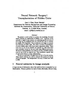
Overall SONOR Architecture and Behavior SONOR deals with the perception and production of metrical pulse sequences, as in other oscillator models of rhythm (Large & Kolen, 1994; McAuley, 1995; Miller et al., 1992), by building the periodicity in as a primitive feature of the basic processing units of the system. The units in SONOR, with the exception of a single input/output unit, are sinusoidal oscillators, each with its own characteristic preferred frequency. Each oscillator responds preferentially to input pulse sequences which are close to its preferred frequency. Metrical patterns characterized by periodicity at multiple levels activate oscillators with preferred frequencies related by integer ratios. The predisposition for metricality takes the form of connections between such oscillators which cause one to tend to excite and couple with the other, all else being equal. The exibility required to handle temporal noise is achieved through phase coupling: the oscillators adjust their phase angles in response to the beats in the input (Large & Kolen, 1994; McAuley, 1995). A SONOR network is a structured collection of such units, each of which repeatedly updates itself until the network stabilizes. Thus it belongs to the family of attractor neural networks rst studied by Hop eld (1982). While such networks grossly oversimplify real neural networks, for example, in their requirement that all weights be symmetric, they appear to be good candidates for investigating some of the abstract global properties of brains (Amit, 1989). A SONOR network is designed to respond to input sequences of pulses when it is in perception mode and to produce output sequences of pulses when it is in production mode. The network has a single input-output (IO) unit representing its simple interface to the world. In perception mode (Figure 1), the IO unit has its output repeatedly clamped to the values of an input sequence of pulses. The other units in the network respond to this pattern. Unlike the IO unit, these other units are oscillators which are naturally activated by periodic inputs. The response of the network to the input sequence depends on (1) the built-in periods of the oscillators and (2) the weights on the connections joining the oscillators to each other and to the IO unit, some or all of which may be learned. In production mode (Figure 2), the oscillators in the network begin with some initial state, normally the state they reached in response to an input sequence during perception mode, and the unclamped IO unit responds to the changing outputs of the oscillators. Long-term knowledge in SONOR, as in other neural network models, takes the form of weights on the connections joining the processing units. These weights are strengthened or weakened as the network responds to particular input patterns, and the network's response to input patterns depends on the weights as well as on the nature of the input. Because all of the connections joining the oscillators are symmetric and because the network's input and output pass through the same unit, perception and production can rely on the same long-term knowledge built into the connection weights. When the IO unit is activated by an input pattern, the system is in perception mode. When the IO unit is free to respond to activation elsewhere within the network, the system is in production mode. Because the weights are adjusted in response to the properties of the input, the network can learn to prefer particular frequency ranges and particular meters and to distinguish particular metrical patterns from one another.

METER AS MECHANISM a

7

Oscillators

Input-output unit

b

Figure 1. SONOR perception mode. The square represents the IO unit, the circles oscillators, the arrows weighted connections. The diameter of each circle represents the preferred period of the oscillator. The IO unit is activated with a periodic pattern, indicated by the curve within the square (a). The IO unit is joined by weighted connections to oscillators. Periodic output from the IO unit causes those oscillators which are consistent with the input pattern to be activated and to give o their own periodic output, indicated by the curves within the circles (b). Since the IO unit is clamped (indicated by the double boundary) it is unaected by the outputs of the oscillators.

SONOR Processing Units Each processing unit in a SONOR network is a standard neural network unit in most ways. It is joined by weighted connections to other units. Unless it is clamped to a particular activation, it repeatedly sums its input and computes an activation, which is a function of the input.

METER AS MECHANISM a

8

Oscillators

Input-output unit

b

Figure 2. SONOR production mode. Certain of the oscillators are activated initially (a), possibly by an input pattern presented to the IO unit. In combination, these activate the (unclamped) IO unit, leading to a periodic output (b).

Oscillators All but one of the units in a SONOR network, the IO unit, are oscillators. We rst consider the behavior of a single oscillator responding to other units in the network (either the IO unit or other oscillators). In most ways the oscillators in SONOR resemble the oscillatory units in two other recent models of rhythm processing, those of McAuley (McAuley, 1995) and Large and Kolen (Large & Kolen, 1994). There are two important dierences. (1) The oscillators in SONOR are connected (coupled) with one another in a neural network, and the weights on the connections in this network are learned. (2) The

METER AS MECHANISM

9

input patterns that the network responds to consist of pulses of varying intensity rather than uniform pulses in particular temporal positions. In what follows, we will treat McAuley's and Large & Kolen's models as reference points for the discussion of SONOR. An oscillator is de ned by its periodic output.4 The output of each oscillator is a sinusoidal function of the time that has elapsed since some initial time t0 . For an oscillator i, it is convenient to express each point in time t as a phase angle i (t), a measure (in radians) of where the oscillator is within its current cycle at t. For a given time t, an oscillator's phase angle depends on its frequency. Each oscillator has a real instantaneous frequency, which may dier from its preferred frequency.5 When the oscillator is unaected by other oscillators, its preferred frequency is equal to its real instantaneous frequency. For an oscillator connected to other activated oscillators, the instantaneous frequency is also aected by phase coupling, which adjusts the phase of an oscillator in response to other oscillators which are at their zero phases, that is, at the peaks of their output functions. Thus an oscillator whose phase angle is =8 when a driving oscillator reaches its phase zero moves its phase angle back to 0 and thereby has its instantaneous frequency decreased, and an oscillator whose phase angle is ?=8 when a driving oscillator reaches its phase zero moves its phase angle ahead to 0 and thereby has its instantaneous frequency increased. Thus the change in phase angle of an oscillator i between two points in time t1 and t2 is the sum of the change due to the oscillator's preferred frequency fi and the change due to phase coupling with other oscillators which reach their zero phases during this interval,
C i (t1;2 ): i(t2 ) ? i (t1) = 2(t2 ? t1)fi +
C i(t1;2): (1) To de ne the precise behavior of an oscillator then, we need to spell out how phase coupling works (the second term on the righthand side of Equation 1) and how output depends on phase angle. As in McAuley's model and in neural networks generally, each oscillator also has a time-varying, but non-periodic activation, a measure of how well the oscillator has synchronized with the other units in the network. A unit's output in SONOR depends on its activation, as we shall see. As in other neural networks, a unit's activation depends in turn on the input to the unit. Thus four equations de ne the behavior of a SONOR oscillator, an input function, an activation function, an output function, and a coupling function. The output of an oscillator peaks at its zero phase and becomes more and more pulse-like as the oscillator becomes active. This re ects the unit's increasing con dence in the placement of its \beat" at its zero phase. The output is also scaled by the oscillator's activation, achieving its maximum value of 1.0 at its zero phase when the oscillator is maximally activated: Oi (t) = Ai(t)[:5 cos(i (t)) + :5] (t) ; (2) i

We will use the terms that are familiar in neural network parlance. These dier to some extent from those used for other oscillator models. Our \output" corresponds to McAuley's \activation;" our \activation" (see below) corresponds to McAuley's \output" and to nothing in Large & Kolen's model. Large & Kolen's \activation" does not map onto anything in SONOR. 5 In models with frequency coupling, as well as phase coupling, we must distinguish an oscillator's xed preferred frequency from its time-varying driving frequency. Frequency coupling adjusts the driving frequency of oscillators in response to the outputs of other oscillators. While we have implemented frequency coupling in SONOR, it will not concern us in this paper, so we will assume that an oscillator's driving frequency is constant and equal to its preferred frequency. 4

METER AS MECHANISM

10

where the exponent i (t), the gain of unit i at time t, determines the sharpness of the output. Gain is a function of activation (as in McAuley's model). For a given activation, we would like the absolute, rather than the relative sharpness, to be constant. Otherwise low-frequency units, with relatively wide beats, would tend to dominate high-frequency units, with relatively narrow beats. Since the units have to work together in real time, their output \pulses" need to be comparable. Therefore, gain in SONOR also depends on the unit's frequency:

i(t) = C (fi)Ai(t); (3) where C is a correction factor which is a function of the frequency of the oscillator. Figure 3 shows the output for a particular low-frequency oscillator at dierent activation values. Output 0.6 0.5

activation=.1 activation=.3 activation=.6 activation=.8

0.4 0.3 0.2 0.1

Pi

-Pi

Phase Angle

Figure 3. Output of an oscillator (preferred period = 2 \time units") at dierent activations.

The periodic pulses of the output of an activated oscillator also de ne the \windows" in which the oscillator responds to the output of other units in the network. Therefore we we will sometimes refer to the oscillator's output function as its response window. An oscillator responds in two ways to other units. First, as in McAuley's and Large & Kolen's models, it adjusts its phase angle in the direction of a pulse it receives from another unit. Second, as in other neural networks but unlike the two oscillator models,6 it adjusts its activation depending on the activation of the units sending it input and on the weights on the connections joining them to it. For activation, the input to the oscillator is: N X I (t) = O (t) [O (t)W i

i

j

j

i;j ];

(4)

where Wi;j is the weight on the connection joining units i and j . Thus the input to a unit is the weighted sum of the outputs of connected units scaled by the unit's response window. The inclusion of the response window in the input function implements the increased attention that is dedicated to points near the unit's phase zero and the increased con dence that comes with the activation of the unit.

6 Activation in McAuley's model (which he calls \output"), is calculated in terms of a memory of previous phase angle adjustments.

METER AS MECHANISM

11

As in other neural networks, an oscillator's activation is a measure of the extent to which it \matches" the current input. In SONOR, matching the current input means synchronizing with the pulses which are output by the other units in the network. The activation function for oscillators is a slightly modi ed version of the familiar activation update rule of the Interactive Activation and Competition model (McClelland & Rumelhart, 1981). In this rule, activation is adjusted at each update as a function of the input to the unit and of decay back to the unit's preferred frequency. The SONOR version incorporates periodicity in both the input and the decay terms. if Ii (t)  0,
Ai (t) = Ii (t)(Amax ? Ai (t)) ? D(Ai (t) ? Arest )(Oi (t))2 :

(5)

if Ii (t) < 0,
Ai (t) = Ii (t)(Ai (t) ? Amin ) ? D(Ai (t) ? Arest )(Oi (t))2 : Here Amax , Amin , and Arest are the maximum, minimum, and resting activations for the oscillators, and D is a decay factor. For the simulations reported here, Amax is 1.0, Amin is 0.0, and Arest is 0.0, and D is 0.1. The inclusion of the response window function in the decay term causes the oscillators to tend to return to their resting activation to the extent that they are activated and near their zero phase. As in the other two oscillator models, an oscillator adjusts its phase angle in response to another unit when that unit's peak pulse (its zero phase) occurs within the oscillator's response window. When an oscillator j reaches its zero phase, the resultant change in the phase angle of oscillator i is given by the oscillator's coupling function:
i (t) = Oi (t)
i (t)
Oj2 (t)
PNj Wi;j j ; k

j Wi;k j

(6)

where i (t) is expressed as a quantity between ? and  radians. Thus when an oscillator receives a pulse within its response window and preceding its zero phase, its phase angle is shifted ahead to 0. When it receives a pulse following its zero phase, its phase angle is shifted back to 0. The magnitude of the shift depends on the height of the response window (Oi (t)) and is scaled by all of the weights into this oscillator so that weights greater than 1.0 do not cause an oscillator to overshoot its zero phase. Note that, for coupling, it is only the magnitudes of the weights that are signi cant. In SONOR, coupling is also constrained by a \refractory period," which prevents phase angle adjustment in an oscillator which has recently reset its phase to zero on the basis of input from another unit. McAuley and Large & Kolen have analyzed the oscillators within their models in terms of the Poincare map, which characterizes the dynamics of a system of two oscillators, a driving and a driven oscillator. In both cases, and for the similar oscillators within SONOR, the long-term behavior of the system is characterized by attractor states in which the oscillators phase lock at integral frequency ratios (1:2, 1:3, 2:3, etc.). The particular behavior of a given system depends on the coupling strength (in SONOR the weight on the connection joining the oscillators), the ratio of the two oscillators' preferred frequencies, and the coupling function itself (Equation 6 for SONOR). The main point is that for a high

METER AS MECHANISM

12

enough coupling strength, oscillators whose preferred frequency ratio deviates considerably from an integral ratio can stabilize at an integral frequency ratio as the driven oscillator is entrained to the driving oscillator, that is, as the phase angle of the driven oscillator is repeatedly aligned in accordance with the pulses of the driving oscillator. With respect to phase coupling, there are two main dierences between SONOR and the other two oscillator models. First, for two coupled oscillators, both are simultaneously driving and driven; that is, each adjusts its phase angle in response to the other. Second, input pulses may come either from the world via the IO unit, or from other oscillators. In the other two models, the inputs are actual pulses from the world; in SONOR they are the pulse-like power-of-cosine outputs of units in the network. However, it is only at their peak response that these units aect the phase angle of other oscillators; that is, the oscillators treat the outputs of other oscillators and the IO unit as pulses. Input/Output Unit The network's single IO unit represents the interface between SONOR's oscillators and the world. Input patterns are presented to the oscillators via this unit in perception mode, and the output of oscillators is ltered through this unit in production mode. The IO unit is distinguished from the other units in the network in several ways. Since it is always clamped during perception mode, its behavior only emerges during production mode. During production we would like it to simply sum and squash the outputs of the network of oscillators. Thus, unlike the other units, the IO unit is not an intrinsic oscillator with a built-in instantaneous frequency of its own. When it outputs a periodic pattern, this is because there are one or more activated oscillators in the network. In this case, its pulse-like oscillatory activation pattern is a consequence of the oscillatory inputs it receives from the oscillators and its high activation decay rate. In perception mode, the IO unit's activation is clamped to a periodic power-of-cosine function representing an external input pattern. This function, which is identical to the output function of the oscillators, implements a periodic sequence of pulses whose widths depend on the exponent of the cosine (Equation 2). Temporal noise may also be added to the input sequence function. Because it is always clamped, the IO unit remains unaected by the rest of the network in perception mode. In production mode (and in the \negative" phase of learning in perception mode, for which see below), the IO unit is unclamped and activated by the oscillators in the network. Input to the IO unit when it is unclamped is the same as it is for oscillators, except that there is no response window:

I (t) = 0

N X [O (t)W i

i

;i ];

0

(7)

where W0;i is the weight on the connection joining the IO unit and oscillator i. The activation update rule for the IO unit is simply the interactive activation rule on which the activation rule for the oscillators was based: if I0 (t)  0,
A0 (t) = I0 (t)(Amax ? A0 (t)) ? D0(A0 (t) ? Arest ): 0 0

(8)

METER AS MECHANISM

13

if I0 (t) < 0,
A0 (t) = I0 (t)(A0 (t) ? Amin ) ? D0 (A0 (t) ? Arest ): 0 0 is -.1, and D0 is 1.0. is -.2, and Arest is 1.0, Amin For the simulations reported here, Amax 0 0 0 The high decay term causes the IO unit's activation to drop quickly to its resting value during production mode when it is not receiving input from oscillators. In this way its behavior during production mode closely resembles its behavior during perception mode, when it is clamped to a pulse-like input pattern. This match between the behaviors of the unit during the two modes is required if Contrastive Hebbian Learning is to succeed (see below). The minimum and resting activations are negative so that oscillators which are not aligned with the pulse of the IO unit are inhibited by it.

SONOR Connectivity With respect to the overall architecture, a SONOR network belongs to the family of settling networks, including Hop eld networks (Hop eld, 1982) and Boltzmann machines (Hinton & Sejnowski, 1986), in which all processing units are joined by symmetrically weighted connections. Oscillators may be connected to other units in one of two ways. A \simple" connection implements a relationship much like that in conventional settling networks. The two units respond continually to each other's activation, which is not periodic. A \coupling" connection implements a periodic relationship between the units; the units respond to each other's periodic outputs . The pattern of simple and coupling connections which is built into a SONOR network is intended to create the potential for hierarchical metrical structure to emerge in the network in response to inputs. In the small networks used in the simulations described below, oscillators with frequencies which are related by ratios of 2 or 3 are joined by coupling connections. With a positive weight on these connections, these pairs of oscillators will tend to become phase-aligned. When such oscillators are activated and phase-aligned with each other, we might say the network is in a \metrical state." Oscillators with other sorts of frequency relationships are joined by simple connections. These permit inhibitory relationships to develop with learning so that particular metrical patterns are more easily distinguished from one another.

Processing in SONOR Processing in the network is similar to that in familiar symmetric networks such as Hop eld networks. The units in the network repeatedly update themselves until the network has settled into a stable state. For conventional symmetric networks, this is a simple matter of halting when the amount of change in the activations of the units due to presentation of a pattern over some period of time falls below some threshold. For a temporal symmetric network such as a SONOR network, the matter is much more complicated; in any case, the behavior of the IO unit should not be expected to stabilize because when one or more oscillators in the network are activated, the activation of the IO unit will be sinusoidal rather than constant. Note that the point is not to assess the stability of the network as an outside observer; if this were the issue, we could make use of familiar stability criteria for limit cycles. The problem is for the network itself to estimate its own stability as it is

METER AS MECHANISM

14

running. We currently have no principled way for it to do this. Intuitively, we would like to treat the network as stable when its response to one period of the input pattern is roughly the same as it was to the previous period. But with no apriori constraint on how long an input period is, there is no obvious way to achieve this. For the time being, we simply run the network for a xed, relatively long number of update cycles and assume that this suces for settling. In practice, this seems to have worked satisfactorily. As already noted, the network can be run in two dierent input/output modes, though the processing algorithm itself is identical in both cases. In perception mode, the IO unit is activated by an input pattern only, and the oscillators in the network respond to it. Oscillators which reach relatively high activations represent expectations that input beats will occur at these units' zero phase angles. Highly activated oscillators whose zero phase angles are aligned with one another represent expectations about relatively strong input beats. In production mode, the network starts with a pattern of activation across the oscillators in the network. Then all of the units, including the IO unit, are allowed to update their activations. As the network settles, the IO unit beats along with the activated oscillators, representing the network's output. Note that the same pattern of activation across a group of network oscillators can represent the system's response to a periodic input pattern or the system's internal state when it is producing a periodic output pattern. Figures 4, 5, and 6 show the outputs of the units in a simple network consisting of two oscillators and the IO unit during production mode. The frequency of one oscillator is twice that of the other, the zero phase of the slower oscillator is aligned with that of the faster oscillator, and all three units are highly activated. In this, and subsequent examples, oscillator periods are described in terms of an arbitrary \time unit." In the simulations of the network, each update cycle represents a small time slice, a discrete approximation to continuous updating. At each update cycle, a unit's phase angle is moved forward an amount which depends on its frequency. In addition, each unit also has the possibility of updating its activation and its phase angle in response to input from other units in the network. On each update cycle all of the units in the network are updated in random order. A \time unit" represents 50 of these update cycles. The two aspects of updating, activation and phase-angle coupling, are described below in turn. Activation Oscillators are repeatedly activated in response to input from the units they are connected to, including the IO unit and other oscillators. Activation works as follows. 1. Input to an oscillator is calculated by summing the activations or outputs of all units connected to the oscillator, each scaled by the weight on the connection. Depending on the kind of connection, the oscillator either receives a periodic output or a non-periodic activation from the other units. If this is a coupling connection, the oscillator also lters the inputs through its periodic response window. Thus along coupling connections, an oscillator only receives input when it is within a region around its zero phase angle (Equation 4). Input to the IO unit is calculated similarly, except that it has no response window (Equation 7). 2. The input to the unit is squashed to a range between the minimum and maximum activation values for the oscillator (Equations 5, 8). The activation decays towards a resting activation. For oscillators decay also depends on the unit's response window.

METER AS MECHANISM

15

Output 1.00 0.80 0.60 0.40 0.20 0.00

Time Units 20

25

30

Figure 4. Output of activated oscillator. An oscillator with period of 1 time unit has been activated by an input pattern with alternating strong and weak beats at a period of 1 time unit. This shows the activation of the oscillator once the input pattern has been turned o. This is the same network as that for Figure 5.

Output 1.00 0.80 0.60 0.40 0.20 0.00

Time Units 20

25

30

Figure 5. Output of activated oscillator. An oscillator with period of 2 time units has been activated by an input pattern with strong beats every 2 time units. This shows the activation of the oscillator once the input pattern has been turned o. This is the same network as that for Figure 4.

METER AS MECHANISM

16

Activation 0.80

0.60

0.40

0.20

0.00 Time Units 20

25

30

Figure 6. Output of IO unit. A network consisting of oscillators with periods 1 and 2 has been activated by an input pattern of alternating strong and weak beats at a period of 1 time unit. What is shown is the output of the IO unit after the input pattern has been turned o. That is, the IO unit is responding to the sum of the outputs of the two oscillators (shown in Figures 4 and 5).

Phase Coupling Oscillators in the network may adjust their phase angles in response to input from the IO unit or from other oscillators to which they are joined by coupling connections. When an oscillator receives input from a unit which has reached a peak and it is not currently at its zero phase angle, its phase angle is shifted in the direction of phase zero by an amount which is proportional to the source unit's output, the current value of the destination unit's own periodic response window, and the magnitude of the weight connecting the two units (Equation 6). Figure 7 illustrates the behavior of a single oscillator in response to an input pattern which has the same underlying frequency as the oscillator's preferred frequency but which starts out =2 radians out of phase from the oscillator and is subject to 10% temporal noise, that is, to deviations from perfect periodicity of as much as 10%. Note that the oscillator's output declines when the pulse from the IO unit is relatively far from its zero phase. This is because the activation of the oscillator depends on the degree of synchronization, and output depends on activation.

Learning in SONOR SONOR is distinguished most signi cantly from other models of rhythm cognition in that it learns. As in other neural networks, learning in SONOR consists in altering the modi able weights in the network in response to input patterns. This represents changes in the network's long-term memory. In SONOR, learning is unsupervised since there is

METER AS MECHANISM

17

Output 0.90 0.80 0.70 0.60 0.50 0.40 0.30 0.20 0.10 0.00 -0.10 Time Units 0

5

10

Figure 7. Phase coupling with noisy input. An input pattern (solid curve) with a period of 1 time unit and subject to 10% temporal noise activates an oscillator (dotted curve) with a period of 1 time unit.

no externally provided target for an input pattern. Rather the network's task is \autoassociation in time"; it attempts to reproduce the input pattern that it is receiving.7 The network reproduces the pattern on the same unit where it is presented, the single IO unit. To test the network's capacity to do this, the IO unit is driven by the pattern long enough for the network to settle. Then the IO unit is disconnected from the input pattern, and the network is allowed to settle again. The network has successfully auto-associated the pattern if the sequence of activations in the network, including the IO unit itself, does not change signi cantly when the IO unit is unclamped. Learning in SONOR is based on the Contrastive Hebbian Learning (CHL) algorithm (Movellan, 1990), a learning algorithm for symmetric settling networks with continuous activation functions. CHL is designed for supervised learning: for each input pattern, the system is also provided with an associated target pattern. As we will see, however, it is straightforward to implement auto-association with CHL. Learning in CHL takes place in two phases, a \positive" phase in which input units are clamped to the input pattern and output units are clamped to the target pattern and a \negative" phase in which only the input units are clamped. In both phases the unclamped units are allowed to settle to Note that other approaches to reproduction of patterns based on spectral decomposition fail because they do not extract phase information. These approaches would miss the invariance in a periodic pattern subject to temporal noise or gradual rate change. 7

METER AS MECHANISM

18

relatively stable activations before the weights are adjusted. During the positive phase, the weight adjustment is Hebbian; that is, each weight is moved an amount which is proportional to the product of the activations of the units on either end of the connection. These changes can be seen as encouraging the associations between correlating input and output units, mediated by the hidden units. During the negative phase, the weight adjustment is anti-Hebbian; each weight is moved an amount which is proportional to the negative of the product of the two activations. These changes can be seen as correcting for spurious associations in the network. For a given input pattern, when the network's weights allow it to accurately reproduce the output pattern, the positive and negative phase weight changes will exactly cancel either other. When this is the case for all of the patterns, the weights will have stabilized. For unsupervised auto-association, as we have implemented it, there are no separate input and output units. This necessitates a minor modi cation to the algorithm. In our positive phase, the IO unit is clamped to a pattern, and in our negative phase, which must follow the positive phase directly, this unit is unclamped (so that no units at all are clamped). If the system has learned the pattern in question, its state will not change when the IO unit is unclamped, and the unit activations will remain as they were during the positive phase. A more signi cant change to the algorithm is necessary because we are dealing with the network's response to patterns in time rather than to the static patterns that are appropriate for the basic CHL algorithm. Thus we are not really clamping the IO unit to a xed value; we are repeatedly clamping it to dierent values. On the one hand, as noted above, this means that we cannot expect anything like stabilization of the network prior to the weight updates. At the very least, the IO unit will continue to change its activation as the pattern is presented during the positive phase or produced by the network during the negative phase. However, as we have seen, it may be possible to simply run the network long enough so that we assume it is as stable as it will get. More seriously, we are faced with the problem of how to adjust the weights. For temporal patterns, weight adjustments need to be based not on the activation co-occurrences at a single point in time but on the pattern of co-occurrences throughout the whole input sequence. For this reason, we accumulate the weight changes for a given pattern over a stretch of time rather than at a single point in time. Again we have the problem of how long the update period should be; it should be long enough to include at least one period of the input pattern, but of course we have no idea how long the period is. We have used the same makeshift approach here as we have for the settling criterion; we simply accumulate weight updates for a stretch of time which is signi cantly longer than the periods of any of the patterns we are likely to deal with. As in the standard CHL algorithm, the weights are not actually updated until the values are accumulated for both the positive and negative phases. The changes are proportional to the sum of these two values for each weight. As in standard Contrastive Hebbian Learning (Movellan, 1990), the weight changes are
Wi;j = L(
Wi;j+ ?
Wi;j? ); (9) where L is a learning rate constant and
Wi;j+ and
Wi;j? are the weight change values accumulated during the positive and negative phases. As with the activation rule, there

METER AS MECHANISM

19

are separate update rules for normal and coupling connections. For normal connections the usual CHL rule applies:
Wi;j (t) = Ai (t)Aj (t): (10) For coupling connections, we modify the standard algorithm to re ect the fact that units only interact with each other when they are near their zero phase angle (or, for the IO unit, near an activation pulse). Thus the value accumulated during each phase depends on the periodic outputs of the units rather than simply on their activations. Between the IO unit and oscillator i, the changes are:
W0;i (t) = A0 (t)Oi (t):

(11)

For the weights on the coupling connections between oscillators, the changes are:
Wi;j (t) = (Ai (t)Oj (t) + Aj (t)Oi (t))

(12)

Learning Simulations In the Assumptions section above, we listed three sorts of learning that should be accomplished by a model of the acquisition of linguistic meter. We now treat each of these in turn and illustrate how a simple SONOR network embodies them. The simulations which we discuss are quite limited and are meant to serve only as demonstrations of the potential of the framework for the learning of meter. In particular, we treat only cases in which the frequency of the metrical levels in the input pattern matches the preferred frequency of oscillators in the network. In a more elaborate model including frequency coupling, as well as phase coupling, we would expect some generalization across dierent pattern frequencies.

Sensitivity to Particular Period Ranges If there is a degree of periodicity in language, it probably occurs at dierent mean frequencies in dierent languages. For example, in Japanese, the mora and the bimora (with periods of roughly 230 and 460 ms) are the best candidates (Tajima, 1998) while in English, the foot or phrase (with periods of at least 500 ms) is a more likely level for periodicity. It also seems possible that nested metrical patterns, that is, those with more than one level, may be more or less dominated by the higher (slower) level. If the slower beats are more regular, a learner should end up more oblivious to deviations at the faster level. Thus if there is periodicity to be found and bene ted from, it is to the learner's advantage to preferentially weight those parts of the rhythm processing system responsible for the frequency range where it occurs. There are two cases to consider: (1) one frequency may occur more often than others; (2) one frequency may occur with less uctuation than others. Simulation 1 addresses the rst, Simulation 2 the second. Patterns with No Nesting: Simulation 1 In Simulation 1, we show how a SONOR network can learn to prefer a frequency which recurs in the input. We treat the simple case in which the input is always an (approximately) isochronous sequence with the same frequency, that is, a metrical pattern with no nesting. For Simulation 1, the network consists of oscillators with periods of 1, 2, and 3 time units, and the network is presented a simple input pattern with a period of 3 time units

METER AS MECHANISM

20

and subject to 5% temporal noise. That is, each event in the noisy pulse train can occur with equal probability anywhere in a window centered around the positon of the ideal, error-free event; the width of this window is 5% of the period of the pulse train. Both the period-1 and period-3 oscillators should respond well to this input pattern, but the period-3 oscillator should be favored because there is an input pulse for each of its zero phase angles. Thus we expect the strongest input-output weight to the period-3 oscillator and the weakest input-output weight to the period-2 oscillator. In addition, the oscillators should learn to inhibit one another, preventing the period-2 oscillator, and to a lesser extent the period-1 oscillator, from responding. In this, and all other simulations, the network was initialized with weights of 1.0 on connections joining the IO unit and oscillators and weights of 0.0 on connections joining oscillators to each other. Figure 8 shows the connectivity of the network and the weights after 20 learning update cycles. The built-in coupling connections between the period-1 and period-2 and between the period-1 and period-3 oscillators re ect the fact that these pairs could participate in metrical patterns. After training, a strong weight has developed to the period-3 unit from the IO unit. This, together with the inhibitory connections among the oscillators, causes the period-3 unit to be highly activated and the other two oscillators to be inhibited in response to the input pattern. The negative weight on the connection between the period-3 and period-1 oscillators requires some explanation since both are consistent with the input pattern and could participate in a nested metrical relationship. However, recall that the network's task is to reproduce the input pattern, and an activated period-1 oscillator would cause output beats at every time step, beats which do not appear in the input pattern. The negative connection between the period-1 and period-3 oscillators causes the period-3 oscillator to overcome the input which the period-1 oscillator receives from the input beats so that this oscillator fails to become activated. Note that if the input pattern had included weaker beats on every time step, the weight between the period-1 and period-3 oscillators would have been greater. Figure 9 shows how the trained network responds after presentation of the pattern when its IO unit is unclamped. Only the activation of the IO unit is shown. The appropriate pattern is produced because only the period-3 oscillator remains active. (The minor

uctuations between the pulses are due to the slight activation of the other two oscillators.) Patterns with Nesting: Simulation 2 In Simulation 1, the network learned to prefer a particular period because it was frequent. But a period could also come to be preferred because it is subject to less temporal noise than other periods. For Simulation 2, the network consists of the IO unit and oscillators of periods 1 and 2. The single input pattern is a nested metrical pattern with strong beats every 2 time units alternating with weak beats (roughly) every 2 time units. The two oscillators that are provided are those which should respond maximally to the periodicities in such an input. The question is which of the two oscillators will learn to respond more strongly to the IO unit and what sort of weight will develop between them. There are two input conditions. In Condition A, both the strong and weak input beats are perfectly periodic. In Condition B, the weak input beats are subject to 5% noise. The patterns are diagrammed in Figure 10 For Condition B, we expect the network to learn to pay more attention at

METER AS MECHANISM

21

Pd=3

.72 -.03

.47

Input/output unit

Pd=2 -.11

-.28

.64

Pd=1

Figure 8. Simulation 1: Learning to respond to a particular frequency. The nal weights in the network are shown. The network consists of the IO unit and three oscillators, represented by circles. Relative circle diameter indicates oscillator period. Arrows with lled heads denote coupling connections; those with un lled heads denote simple connections. Along each connection is shown its nal weight after the network has been trained on inputs with a period of 3 time units.

the period-2 level than the period-1 level because every other beat is perfectly predictable. For Condition A there should be no advantage for the period-2 level because the beats are perfectly predictable at both periods. Figure 11 shows weights for the two conditions after 30 learning update cycles. For Condition A, the weights to the period-1 oscillator are slightly higher, while for Condition B, as predicted, the weights to the period-2 oscillator are higher. In addition, the weight connecting the oscillators is negative for Condition B, re ecting the inconsistent relation between them. Thus a deviant weak beat can cause the period-1 oscillator to expect the next (strong) beat too early or too late and, at least temporarily, to fail to synchronize with the period-2 oscillator. Under both conditions, however, the network is able to reproduce the metrical input pattern once it has been turned o. The output of the unclamped IO unit for the trained network in Condition B is shown in Figure 12. It can be seen that the IO unit reproduces both the period-1 and period-2 beats.

Sensitivity to Particular Meters: Simulation 3 In Simulation 2, we saw that the network could learn to reproduce a metrical pattern. Various kinds of simple music employ particular metrical structures, for example, strong stresses on every second rather than every third beat. Learners who can gure this regularity

METER AS MECHANISM

22

Output

0.20 0.15 0.10 0.05 0.00 -0.05 -0.10 Time Units 20

30

40

Figure 9. Simulation 1: Learning to respond to particular frequency. The network is that shown in Figure 8. After training, the IO unit is driven by an input pattern of period 3, then allowed to vary in response to the outputs of the oscillators. The output of the IO unit beginning at this point is shown.

out are in a better position to direct their attention to the strong stresses. For Simulation 3, the network is the same as that in Simulation 1. That is, there are oscillators with periods of 1, 2, and 3 time units. The input pattern consists of alternating strong and weak beats, each with a period of 2, identical to the patterns in Simulation 2, Condition A (Figure 10). We expect the period-1 and period-2 oscillators to respond best to the pattern, and this should be re ected in a small weight from the IO unit to the period-3 oscillator following training. The network should develop an inhibitory connection between the period-2 and period-3 oscillators in order to exaggerate the dierence between the duple and triple meters. Figure 13 shows the weights after 30 update cycles. The period-3 unit has the predicted weak connection from the IO unit and is inhibited by both other oscillators. Figure 14 shows the response of the trained network after it has been presented with the input pattern and then unclamped. We see that the network reproduces the pattern appropriately. Analogous results are obtained when the network is trained with a triple, instead of a duple meter.

METER AS MECHANISM

23

Intensity

A

0

1

0

1

2 3 Time (in time units)

4

5

4

5

Intensity

B

2 3 Time (in time units)

Figure 10. Simulation 2: Input patterns. In Condition A, there are strong pulses every 2 time units alternating with weak pulses every 2 time units. Condition B is the same, except that the weak beats are subject to temporal noise. Pd=2 A: .82 B: 1.0 A: .17 B: -.66

A: .94 B: .89

Pd=1

Figure 11. Simulation 2: Learning to respond to noise-free frequency. The nal weights are shown. The network consists of the IO unit and two oscillators. There were two dierent training conditions. In Condition A, a noise-free duple pattern was presented. In Condition B, a duple pattern with 5% temporal noise on the weak beats was presented. Final weights for both conditions are shown.

METER AS MECHANISM

24

Output 0.80 0.70 0.60 0.50 0.40 0.30 0.20 0.10 0.00 -0.10 Time Units 20

25

30

35

Figure 12. Simulation 2: Learning to respond to noise-free frequency. The network shown in Figure 11 is trained in Condition B. Following training the network is presented with another noisy duple input pattern; the IO unit is then allowed to vary freely in response to the activated oscillators. The output of the IO unit beginning at this point is shown.

Selectivity to Particular Meters: Simulation 4 Many languages, English, for example, make use of a variety of metrical structures. If we assume a tendency for a particular meter to persist, as is certainly the case in music and verse, then it is to the advantage of listeners to be able to identify which meter is being used after a relatively small number of repetitions so that they can make use of expectations based on the meter. And it is to the advantage of learners to gure out how to do this. For Simulation 4, the network consists of the IO unit and oscillators with periods of 1, 1.5, and 3 time units. There were two sorts of input patterns, and the network was trained separately on them. That is, it was not expected to shift to one pattern after entraining to the other. Pattern A had strong beats every 3 time units and weak beats midway between every pair of strong beats, a duple meter. Pattern B also had strong beats every 3 time units, but there were 2 weak beats for every strong beat, subdividing the intervals separating the strong beats into thirds rather than halves, a triple meter. Thus Pattern A favors the period-1.5 oscillator and Pattern B favors the period-1 oscillator while both patterns are consistent with the period-3 oscillator. The patterns are diagrammed in Figure 15. As before, we start the network up with positive weights on connections joining the IO unit to the oscillators and weights of 0.0 on the inter-oscillator connections. We might expect

METER AS MECHANISM

25

Pd=3

-.04

Pd=2

.05

.82

-.23

.94 .25

Pd=1

Figure 13. Simulation 3: Learning to respond to a particular meter. The nal weights are shown. The network consists of the IO unit and two oscillators. The network was trained only on duple input. Final weights are shown for each connection.

this con guration to permit the inputs to be distinguished, but all of the oscillators are highly activated when either input pattern is presented. Figure 16 shows the response of the unclamped IO unit after presentation of the duple pattern to the untrained network. The output is a useless combination of the duple and triple patterns. The same behavior results when the triple pattern is input. Training should adjust the IO-to-oscillator connections and create an inhibitory connection between the period-1 and period-1.5 oscillators. The result should be a network with an attractor state for each of the two input patterns. Figure 17 shows the weights after 10 update cycles. The major changes are in the pattern of weights on the inter-oscillator connections. A weak inhibitory connection has developed between the period-1 and period-1.5 units. The inhibitory connection joining the period-3 and period-1 units apparently functions to adjust the relative activations of these units when both are active. In any case, the weight changes now permit the network to respond selectively to the two input patterns. As shown in Figures 18 and 19, each pattern is correctly reproduced on the IO unit when it has been presented and then removed. With this simulation, we have shown that a network without the initial ability to distinguish metrical input patterns can develop this selectivity simply by being repeatedly exposed to the dierent patterns. The network's power comes from auto-association. Given an input pattern, it adjusts its weights in such a way that it can reproduce that pattern better.

METER AS MECHANISM

26

Output 0.80 0.70 0.60 0.50 0.40 0.30 0.20 0.10 0.00 -0.10 Time Units 20

25

30

35

Figure 14. Simulation 3: Learning to respond to a particular meter. The network is the one shown in Figure 13. After training, the IO unit is driven by an input pattern with duple meter, then allowed to vary. The output of the IO unit at this point is shown.

Conclusions and Future Work While the SONOR model is only a rst step towards a full-blown computational account of the learning of linguistic or musical metrical patterns, it already permits several predictions about the processing of meter by human subjects. 1. The model performs best on patterns resembling those it was trained on. This holds for the kind of meter, as well as the frequency, of the patterns. Thus the model predicts that long-term exposure to triple meter results in an enhanced performance on various tasks that we might devise, e.g., detecting deviations from periodicity on triple patterns, distinguishing triple patterns from duple patterns, predicting beat locations within triple patterns. Each of these tasks can be realized in a straightforward way within the model. Deviations from periodicity are re ected in the lowered activations of units. The extent to which the network distinguishes two sorts of meter is re ected in the dierent output it produces when \replaying" dierent patterns following exposure to them. Predictions regarding beat locations are re ected in the timing of the phase zeros of activated oscillators. 2. A SONOR network consists of a bank of oscillators, each responding to a range of frequencies around its preferred frequency. Given long-term exposure to periodicity at a particular narrow frequency range, a single oscillator develops strong connections to the

METER AS MECHANISM

27

Intensity

A

0

1

2

3

0

1

2

3

4 Time (in time units)

5

6

7

8

5

6

7

8

Intensity

B

4 Time (in time units)

Figure 15. Simulation 4: Input patterns. In Condition A, there are strong pulses every 3 time units alternating with weak pulses every 3 time units (a duple meter). In Condition B, there are strong pulses every 3 time units, and between each pair of strong beats there are two evenly spaced weak beats (a triple meter).

IO unit, and the network later responds more readily to patterns near that frequency.8 Frequency coupling (not discussed in this paper, but implemented in SONOR) permits generalization to patterns at frequencies other than those in the training set, but frequency coupling is thrown o by frequencies which are roughly 25% greater or less than the preferred frequency of an excited oscillator because the input pulses tend to fall outside the input window of the oscillator. While the precise range within which generalization can occur depends on the values of several parameters, generalization breaks down rather catastrophically at a point which is less than a 50% deviation from the mean frequency of the training set. Thus the model predicts that subjects will be better able to detect deviations from periodicity (frequency changes or temporal noise) within the range of the training set than far from it. It also predicts a relatively sudden drop in performance as the frequency of test patterns becomes further from that of the training set. An obvious next step is to train the model on pulses generated from real speech. Initially we will try metrically constrained speech such as verse, chants, or \over-rehearsed" speech, such as group prayers. Note that in real biological systems, the tendency to prefer particular frequencies may also depend on built-in preferences of one sort or another (Handel, 1989). 8

METER AS MECHANISM

28

Output 1.00 0.90 0.80 0.70 0.60 0.50 0.40 0.30 0.20 0.10 0.00 -0.10 Time Units 20

30

40

Figure 16. Simulation 4: Selectivity to meter. The network is the one shown in Figure 17 with initial weights of 1.0 on connections to and from the IO unit and 0.0 elsewhere. The IO unit is driven by a duple input pattern, then allowed to vary freely. The output of the unit at this point is shown.

Before we are ready for the rhythm of actual speech, however, several aspects of the model need more investigation. Some of these have to do with coupling. Currently frequency coupling is confused by minor deviations from perfect periodicity, and phase coupling has diculty recovering from a tendency to couple too strongly with an initial beat that happens to be followed by a stronger one. Others have to do with learning. We need to establish that the model is capable of acquiring more complex rhythms, for example, meters with three levels, patterns with alternating meters, or periodic patterns containing rests (Gasser & Eck, 1996). We also need a principled way of