A Review of Regression Models Employed for Predicting Diffuse Solar ...

Trends in Renewable Energy Peer-Reviewed Article

OPEN ACCESS ISSN: 2376-2144 futureenergysp.com/index.php/tre

A Review of Regression Models Employed for Predicting Diffuse Solar Radiation in North-Western Africa Ogbulezie Julie C.1, Ushie Ogri James2, Nwokolo Samuel Chukwujindu1* 1

Department of Physics, Faculty of Physical Sciences, University of Calabar, Nigeria, P.O. Box 2892, Calabar, Nigeria 2 Department of Electrical/Electronic Engineering, Faculty of Engineering, University of Calabar, P.O. Box 2892, Calabar, Nigeria Received September 28, 2017; Accepted November 14, 2017; Published November 14, 2017 The knowledge of diffuse solar radiation (Hd) is of almost importance for determining the gross primary productivity, net ecosystem, exchange of carbon dioxide, light use efficiency and changing colour of the sky. However, routine measurement of Hd is not available in most locations in North-Western Africa. During the past 36 years in order to predict Hd in the horizontal surface on hourly, daily and monthly mean basis, several regression models have been developed for numerous locations in NorthWestern Africa. As a result, several input parameters have been utilized and different functional forms applied. The regression models so far utilized were classified into six main categories and presented based on the input parameters applied. The models were further reclassified into numerous main groups and finally represented according to their developing year. In general, 188 regression models, 33 functional forms and 20 groups were reported in literature for predicting Hd in NorthWestern Africa. The regression and soft computing models developed within North-Western Africa and across the globe were examined in order to determine the best technique of prediction. The result revealed that soft computing models are more suitable for predicting Hd in North-Western Africa and across the globe. Keywords: Diffuse solar radiation; Regression models; Classification; Functional forms; North-Western Africa

1. Introduction As a result of exponentially increasing costs of fossils, uncertainty of availability and transportation, environmental pollution, and general awareness amongst common people, the renewable sources which are environmental friendly since they have much lower environmental impact compared to conventional sources have enabled smart energy to gain more attention from researchers, governments, non-governmental organisations (NGOs) and industries etc. in recent years due to the rapid growth of the global energy demands. Solar energy in the form of radiation received at the surface of the earth is the most preferred sustainable source of renewable energy in the form of solar photovoltaic, solar thermal. Other sources of renewable energy are wind, biomass, small and big hydro, tidal, wave, ocean etc. as a result of their inexhaustible nature and abundant availability globally. These attributes make solar energy to be accepted worldwide as a key energy *Corresponding author: [email protected] Tr Ren Energy, 2017, Vol.3, No.2, 160-206. doi: 10.17737/tre.2017.3.2.0042

160

Peer-Reviewed Article

Trends in Renewable Energy, 3

source for the future with respect to the environmental issues associated with fossils as well as their limited reserves. Therefore, solar energy is the best substitute of fossils owing to the ever growing demand for energy globally. In fact, about 40 GW of solar photovoltaics (PV) capacity was installed in 2014 and the International Energy Agency, IEA [1] predicts that by 2050, photovoltaic (PV) as a renewable energy source (solar energy) may become one of the most promising sources of energy that will provide about 11% of global electricity production and would reduce 2.3 gigatonnes of CO2 emissions per year. As a result, more and more penetration of solar energy technologies to the worlds’ energy sector is indeed appealing for supplying a notable part of the electricity, heating, cooling, cooking, and drying of all types of things: clothes, agricultural produce, cash crops, and bricks etc. Therefore, a good working knowledge of available solar energy obtained principally from global solar radiation with its diffuse and direct components in a particular location are of great importance in designing and sizing of solar energy conversion systems. Diffuse solar radiation is the component of global solar radiation reaching the earth’s surface after having been scattered from the direct horizontal irradiation by molecules, aerosols or suspended particular matter such as black carbon, organic carbon, dust and sea salt in the atmosphere. Diffuse solar radiation plays an important role in determining the gross primary productivity, net ecosystem exchange of carbon dioxide, light use efficiency, changing colour of the sky and baseline for estimating and understanding diffuse solar radiation parameters such as diffuse solar radiation and global solar radiation on surfaces, diffuse photosynthetically active radiation etc. Moreover, solar energy among other sources of renewable energy has remained the most viable source of energy that has the capacity to sustain and maintain all the activities and processes that support life of animals, supply heat to the atmosphere and lands, generate its wind, drive the water cycle, warm the ocean and support life of plants. The accurate determination and clear understanding of the diffuse solar radiation parameters is required for many applications such as energy management, solar energy, light studies, architectural research, hydrological process and biometeorology, crop production, remote sensing of vegetable and carbon cycle modelling, designing and sizing photovoltaic systems, development of thermal and electrical solar energy devices [2-6]. Diffuse solar radiation arises as a result of the interaction between the solar radiation incident on the top of the earth’s atmosphere and the matter within it. Thus, understanding how this radiometric flux interacts with the matter within it and relates with its immediate environment thereby influencing diffuse light availability for energy, sky colour, agricultural, material and technological production and utilization for man’s need is of utmost importance for modelling and estimating diffuse solar radiation in a particular geographical environment. Diffuse solar radiation varies from one geographical location to another. It is a function of meteorological parameters such as evaporation, effects of cloudiness, relative humidity, precipitation, temperature, sunshine duration, extraterrestrial solar radiation, and reflection of the environs; geographical parameters such as latitude, longitude and elevation of the site; geometrical factors such as azimuth angle, sun azimuth angle; astronomical parameters like solar constant, earth-sun distance, solar declination and hour angle; physical parameters such as scattering air molecules, water vapour content, scattering of dust and other atmospheric constituents like O2, N2, CO2, and O. Measurement of diffuse solar radiation is often performed in many parts of the world by mounting a pyranometer on the axis of the ring on a roof top so as to receive only diffuse solar radiation and the ring is normally adjusted regularly to ensure that the direct Tr Ren Energy, 2017, Vol.3, No.2, 160-206. doi: 10.17737/tre.2017.3.2.0042

161



irradiance does not reach the pyranometer. As a result of cost of measuring equipment, its maintenance and calibration requirements, in rural and developing countries in Africa and several places around the world, several empirical models had been developed in Africa and other locations across the globe that can produce diffuse solar radiation data without the substantial cost of the instrumentation network that would otherwise be needed [7-10]. The most primitive model for estimating diffuse solar radiation was developed by Liu and Jordan [11]. These solar energy researchers correlated diffuse fraction (Hd/H) with clearness index (kt). Their investigation has been adopted by numerous solar energy researchers in Nigeria and Egypt and across the globe as a baseline further developing regression models for estimating diffuse solar radiation using the same parameter, other meteorological parameters, geographical parameters, geometrical parameters and astronomical parameters that will best fit the local climate of their study. However, diffuse solar radiation and other components of solar radiation such as direct normal irradiance, photosynthetically active radiation, evapotranspiration etc. have been predicted employing different soft computing techniques in recent times. This constitutes a widely accepted technique offering an alternative way to synthesize complex problems associated with solar energy prediction. These problems include inability to handle non-linear relationships in data; applying only calculable atmospheric, meteorological, astronomical, geographical, geometrical parameters such as extraterrestrial solar radiation, latitude, altitude, longitude, maximum sunshine duration, azimuth angle, solar declination, cosine of solar zenith angle, and hour angle. The soft computing technique has the capacity of accepting many input parameters for a particular model which is not possible applying regression technique and this strengthens its reliability. Therefore, applying soft computing techniques compared to regression techniques according to previous studies offers greater accuracy with prediction error in a range (less than 20 %) and could be very good in terms of diffuse solar radiation prediction as more and more soft computing approaches are demanded in the domains of renewable energy resource prediction [12-21]. Therefore, the main purpose of the study was to review regression models fitted in literature for predicting diffuse solar radiation in North-Western Africa and its objectives are identifying several input parameters and functional forms ever applied for predicting diffuse solar radiation in North-Western Africa; classify the regression models commonly employed in this part of Africa according to the main input parameters; compare the performance of regression and soft computing models applied and decide the best technique that can yield high accuracies of estimation for future purposes and finally identify the research gap. 2. Basic Parameters The principal parameter of sunshine duration fraction, daily extraterrestrial radiation on the horizontal surface is significant for the prediction of diffuse solar radiation. Sunshine duration fraction is the ratio of actual sunshine duration to maximum possible sunshine duration expressed theoretically as: So 

2 cos1  tan  tan   15

Tr Ren Energy, 2017, Vol.3, No.2, 160-206. doi: 10.17737/tre.2017.3.2.0042

(1)

162



 360n  284  365 

  23.45 sin 

(2)

Where  is the latitude,  is the solar declination given by Yaniktepe and Genc [22] and n is the number of days of the year starting from first January. The daily extraterrestrial solar radiation is the solar radiation intercepted by horizontal surface during a day without the atmosphere and hourly extraterrestrial radiation has similar definition. Hourly extraterrestrial solar radiation on the horizontal surface is given by Zhang et al. [23] as: 12  3600  I SC   (   )  360n   Io  1  0.033 cos    cos cos (sin 2  sin 1) sin S  2 1 sin  sin   (3)  365   180   While the daily extraterrestrial solar radiation on the horizontal surface is given by Yaniktepe and Genc [23] as: Ho 

24



 

I SC  1  0.033 cos

2 S   sin  sin      cos cos  sin  S  365   360 

360n 

(4)

Where the mean sunrise hour angle s  can be evaluated as:

s  cos1  tan  tan  

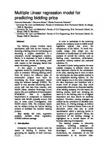
(5) ISC is the solar constant, 1 and 2 are the limit hour angle of an hour, in which 2 is the larger, all in degrees and other symbols retain their usual meaning. 3. Evaluation Metrics Evaluation, principally compares how well the observed and predicted fit each other. This evaluation is applied at numerous steps of the computing model development as for instance during the evaluation of the prediction model itself (during the training of a statistical model for instance), for judging the improvement of the computing model after some modifications and for comparing numerous computing models. As previously mentioned, this performance comparison is not easy for numerous reasons such as different predicted time horizons, numerous time scales of the predicted data and variability of the meteorological conditions from one site to another one. It works by comparing the predicted outputs 𝑦̂ with observed data y which are also measured data themselves linked to an error (or precision) of a measure. Graphic tools are available for predicting the adequacy of the computing model with the experimental measurements via: 1. Time series of predicted diffuse solar radiation in comparison with measured diffuse solar radiation which allows visualizing easily the estimation quality. In Fig. 1a, for instance, high estimate accuracy in clear-sky conditions and a low one in partly cloudy conditions can be seen. 2. Scatter plots of estimated over measured diffuse solar radiation(as shown in Fig. 1b) which can reveal systematic bias and deviations depending on the diffuse solar radiation conditions and show the range of deviations that are related to the estimates. 3. Receiver Operating Characteristic (ROC) curves which compare the rates of true positives and false positive. Tr Ren Energy, 2017, Vol.3, No.2, 160-206. doi: 10.17737/tre.2017.3.2.0042

163



a)

b)

c)

Fig. 1. a) Time series of predicted and measured global radiation for 2008 in Ajaccio (France); b) Scatter plot of predicted vs. measured global radiation in Ajaccio (France); c) Example of ROC curve (an ideal ROC curve is near the upper left corner).

Up till now, there is no standard evaluation measures accepted for diffuse solar radiation measurement, which makes the comparison of the estimating methods difficult. Sperati et al. [24] presented a benchmarking exercise within the framework of the European Actions Weather Intelligence for Renewable Energies (WIRE) with the purpose of evaluating the performance of state of the art computing models for short term renewable energy prediction or forecasting. This research is a very good example of reliability parameter utilization. They concluded that: “More work using more test cases, data and computing models needs to be performed in order to achieve a universal overview of all possible conditions. They also pointed out that test cases located all over Europe, the US and other relevant countries should be considered, in an effort to represent most of the possible meteorological conditions”. This study therefore illustrates very well the difficulties of performance comparisons encountered for diffuse solar radiation prediction. The commonly applied statistics for diffuse solar radiation prediction include the following: The Mean Bias Error (MBE) represents the mean bias of the prediction: 1 N MBE     yˆ i   y i  (6) N i1 𝑦̂ is the predicted diffuse solar radiation, y the measured diffuse solar radiation and N the number of observations. The prediction will under-estimate or over-estimate the observations. Thus, MBE is not a good statistical indicator for the reliability of a computing model because the errors compensate each other but it allows seeing how much it overestimates or underestimates. Tr Ren Energy, 2017, Vol.3, No.2, 160-206. doi: 10.17737/tre.2017.3.2.0042

164



The Mean Absolute Error (MAE) is appropriate for comparing diffuse solar radiation estimation with linear cost functions, i.e., where the costs resulting from a poor prediction are proportional to the estimation error: 1 N MAE    yˆ i   y i  (7) N i1 The mean square error (MSE) applies the squared of the difference between observed and estimated data. This statistical indicator penalizes the highest gaps: MSE 

N 2    yˆ i   y i  N i 1 1

(8)

MSE is principally the statistical parameter which is minimized by the training algorithm. The Root Mean Square Error (RMSE) is more sensitive to big prediction errors, and thus is good for applications where small errors are more tolerable and larger errors cause disproportionately high costs, as in the case of utility applications (http://www.cost.eu/about_cost). It is probably the reliability parameter that is most appreciated and employed: RMSE  MSE 

N 2    yˆ i   yi  N i1 1

(9)

The Mean Absolute Percentage Error (MAPE) is close to the MAE but each gap between observed and predicted value is divided by the observed value so as to consider the relative gap. MAPE 

N yˆ i   yi   N i1 y (i ) 1

(10)

This statistical indicator has a challenge that it is unstable when y(i) is near zero and it cannot be defined for y(i)=0. Of recent, these errors are normalized particularly for the RMSE; as reference the mean value of global radiation is generally employed but other definitions can be applied: N 2    yˆ i   y i  N i1 y 1

nRMSE 

(11)

With 𝑦̅ is the mean value of y. Other statistical indicators exist and can be employed as the correlation coefficient (R), coefficient of determination (R2), or the index of agreement (d) which is normalized between 0 and 1. As the prediction accuracy strongly depends on the location and time period applied for evaluation and on other parameters, it is difficult to evaluate the quality of estimation from accuracy metrics alone. Then, it is best to compare the accuracy of different estimations against a common set of test data Pelland et al. [25]. “Trivial” prediction approach can be applied as a reference [26], the most common one is the persistence model (“things stay the same”, Trapero et al., 2015) where the prediction is always equal to the last known data point. The diffuse solar radiation has a deterministic component due to the geometrical path of the sun. This characteristic may be included as a constraint to the simplest form of persistence in considering as an example, the measured data of the previous day or the previous hour at the same time as a prediction value. Other common reference forecasts include those based on climate constants and simple autoregressive methods. Such comparison with referenced NWP computing model is shown in Fig. 2. Generally, after 1 hour the forecast is better than persistence. For forecast horizons of more Tr Ren Energy, 2017, Vol.3, No.2, 160-206. doi: 10.17737/tre.2017.3.2.0042

165



than two days, climate averages show lower errors and should be preferred for diffuse solar radiationprediction.

Fig. 2. Relative RMSE of forecasts (persistence, auto regression, and scaled persistence) and of reference models depending on the forecast horizon Lauret et al. [27].

Classically, a comparison of performance is performed with a reference computing model and to do it, a skill factor is employed. The skill factor or skill score defines the difference between the forecast and the reference forecast normalized by the difference between a perfect and the reference forecast Lauret et al. [27]: SkillScore 

Metric forecasted  Metricreference Metric perfectfoecast  Metricreference

 1

MSE forecatd

(12)

MSEreference

Its value thus ranges between 1 (perfect forecast) and 0 (reference forecast). A negative value indicates a performance which is even worse compared to the reference (observed data). Skill scores can be adopted not only for comparison between observed and predicted diffuse solar radiation values but also for inter-comparisons of different diffuse solar radiation prediction techniques. 4. Regression Models A regression model relates diffuse solar radiation (Hd) with other easily measurable parameters such as clearness index, mean daily extraterrestrial solar radiation, sunshine fraction and cloud cover by applying concise mathematical functions. As a result of its simplicity and high operability, the regression model is much more convenient for engineering applications. Several regression models have been reported in literature for prediction Hd on the horizontal surface either on hourly mean basis (HB) or daily mean basis (DB) or monthly mean daily basis (MB) in Nigeria and Egypt. In this review, the Hd models are classified according to the basis of their input parameters applied in correlating with either diffuse fraction (Hd/H) or diffuse coefficient (Hd/Ho). It has been accepted that Hd is relatively affected by meteorological parameters, astronomical factors, geographical factors, and geometrical factors [7, 9, 28-29]. This could be attributed to the uniqueness of local climate in determining the meteorological and Tr Ren Energy, 2017, Vol.3, No.2, 160-206. doi: 10.17737/tre.2017.3.2.0042

166



atmospheric parameters that best fit that particular locality. This also depends on the availability of input meteorological/atmospheric parameter(s) that a given radiometric station or an individual is capable of measuring routinely which finally turns out to be the best input parameter at the disposal of the researcher for predicting Hd in that location factors [7, 9]. Thus, in North-Western Africa, the models for predicting Hd can be classified into six (6) following categories based on the employed meteorological and atmospheric parameters via: 1. Clearness index-based models 2. Sunshine-based models 3. Cloud-based models 4. Extraterrestrial Solar Radiation-based models 5. Monthly-based models 6. Hybrid Parameter-based models 4.1 Clearness Index-Based Models The clearness index (kt) indicates the percentage depletion by the sky of the incoming solar radiation and therefore gives both the level of availability of solar radiation and changes in the atmospheric condition in a given environment [8, 30-32]. Mathematically, clearness index is the ratio of horizontal global solar radiation to the extraterrestrial solar radiation (Ho) on daily or monthly basis as found in literature expressed as: kt 

H

(13)

Ho

For this reason, clearness index is closed related to Hd, hence, it has been known as a determinant parameter for estimation of Hd. One of the greatest characteristics of the models from this class is their convenient application, since for utilizing them only measured H data is needed. Numerous functional forms (exponential form, logistic form, logarithm form, second order, third order and power form) have been applied for estimating HB, DB and MB diffuse horizontal irradiation in literature are introduced according to their developing year under this section. 4.1.1 Group 1 Empirical models from this group are parameterized as the first-order polynomial function of the clearness index according to their functional forms and developing year. The functional forms are as follows:  H Hd  a  b Ho  Ho

    H  Hd   a  b H  Ho 

H  Hd  a  b  H  Ho   H H d  a  b  Ho

(14) (15)

1

  

(16) (17)

Ezekwe and Ezeilo [33] developed the following MB models in Nsukka Tr Ren Energy, 2017, Vol.3, No.2, 160-206. doi: 10.17737/tre.2017.3.2.0042

167



For January to May  H Hd  1.13  1.48 H  Ho

  

(18a)

For dry season  H  Hd   1.14  1.69 H H o  

(18b)

Said and Ibrahim [34] developed the following MB model for Cairo, Egypt as:  H Hd  0.86  0.86 H  Ho

  

(19)

Maduekwe and Chendo [35] developed HB diffuse solar radiation for Lagos as:  H Hd  1.021 0.151 H  Ho

    H  Hd   1.385  1.396 H  Ho 

 H    0.30 0    Ho   H    0.80 0.30    Ho 

(20a) (20b)

Babatunde and Aro [36] established the following MB model for Ilorin as:  H Hd  0.945  0.97 H  Ho

  

(21)

Maduekwe and Chendo [37] proposed the following HB models for Lagos  H Hd  1.021  1.151 H  Ho

    H  Hd   1.385  1.396 H  Ho 

 H  (22a)   0.30 0    Ho   H    0.80 (22b) 0.30    Ho 

Trabea [38] obtained the following MB model for AL-Arish, AL-Tahrir, Marsa Matroh, Cairo, Al-Kharga and Aswan located in Egypt as:  H  Hd   0.924  0.894 H  Ho 

(23)

Maduekwe and Garba [39] developed the following HB models for Lagos and Zaria with the appropriate intervals as: For Zaria  H Hd  1.009  0.273 H  Ho

    H  Hd   1.077  1.136 H H o  

 H   Ho

   0.18   H    0.68 0.18   H o  

(24a) (24b)

For Lagos  H Hd  1.002  0.028 H  Ho

    H  Hd   1.336  1.369 H  Ho 

 H   Ho

   0.20   H    0.78 0.20    Ho 

(24c) (24d)

Shaltout et al. [40] developed the following MB models for Cario and Aswan in Egypt. For Cario Tr Ren Energy, 2017, Vol.3, No.2, 160-206. doi: 10.17737/tre.2017.3.2.0042

168



 H Hd  0.93  1.08 H  Ho

  

(25a)

  

(25b)

For Aswan  H Hd  1.01  1.16 H  Ho

El-Sebaii and Trabea [41] developed the following MB models for four Egyptian locations’ For Matruh  H Hd  1.299  1.435 H  Ho

  

(26a)

  

(26b)

For Al-Arish  H Hd  1.377  1.550 H  Ho

For Rafah  H Hd  1.257  1.531 H  Ho

(26c)

  

For Aswan  H  Hd   0.580  0.339 H  Ho 

(26d)

Burari [42] developed the following MB models for Bauchi as follows:  H Hd  0.775  0.804 H  Ho

  

(27)

Ugwuoke and Okeke [43] developed the following models for Nsukka as:  H H d  0.137255 0.1143  Ho

  

(28)

Khalil and Shaffie [44] established the following HB models for Cario, Egypt as:  H Hd  5.817  6.517 H  Ho

  

(29)

Okundamiya et al. [45] established the following MB models for six Nigerian locations For Sokoto  H Hd  1.0658  1.2566 H  Ho

  

(30a)

  

(30b)

  

(30c)

  

(30d)

For Maiduguri  H Hd  1.0600  1.2526 H  Ho

For Abuja  H Hd  1.0506  1.2461 H  Ho

For Ikeja  H Hd  1.0467  1.2461 H  Ho


169



For Enugu  H Hd  1.0454  1.2467 H  Ho

  

(30e)

  

(30f)

For Benin City  H Hd  1.0387  1.2419 H  Ho

Nwokolo and Ogbulezie [10] developed the following MB models for all sky and clear sky in numerous stations in six tropical ecological zones in Nigeria. For Port Harcourt (All sky)  H   H d  14.273  13.50  Ho 

(31a)

For Port Harcourt (Clear sky)  H   H d  1.874  16.922  Ho 

(31b)

For Owerri (All sky)  H H d  10.814  7.031  Ho

  

(31c)

 H   H d  5.400  23.21  Ho 

(31d)

For Owerri (Clear Sky)

For Ibadan (All sky)  H H d  12.059  9.542  Ho

  

(31e)

For Ibadan (Clear Sky)  H   H d  7.4955  26.902  Ho 

(31f)

For Abuja (All sky)  H   H d  14.076  13.008 H  o

(31g)

For Abuja (clear sky)  H   H d  35.705  49.757  Ho 

(31h)

For Maiduguri (All sky)  H   H d  18.049  19.256  Ho 

(31i)

For Maiduguri (clear sky)  H H d  33.121 45.136  Ho

  

(31j)

For Sokoto (All sky)


170



 H H d  19.008  20.404  Ho

  

(31k)

 H   H d  7.8579  3.1059  Ho 

(31L)

For Sokoto (Clear sky)

4.1.2. Group 2 Empirical models from this group are parameterized as the second-order polynomial function of the clearness index according to their functional forms and developing year. The functional forms are as follows:

H  H  Hd   c   a  b H  Ho   Ho 

2

(32)

Trabea [38] obtained the following MB model for AL-Arish, AL-Tahrir, Marsa Matroh, Cairo, Al-Kharga and Aswan located in Egypt as:

H  H  Hd  0.534  0.384   1.0366  H  Ho   Ho 

2

(33)

El-Sebaii and Trabea [41] developed the following MB models for four Egyptian locations’ For Matruh

H  H  Hd   15.439   4.914  18.170 H H H  o  o

2

(34a)

For Al-Arish

H  H  Hd   14.778   4.138  16.540 H H H  o  o

2

(34b)

For Rafah

 H   H  Hd   3.312   2.635  5.652 H  Ho   Ho 

2

(34c)

For Aswan

H  H  Hd  10.45  29.47   21.459  H  Ho   Ho 

2

(34d)

Burari [42] developed the following MB models for Bauchi as follows:

H  H  Hd  0.908  1.31   0.474  H  Ho   Ho 

2

(35)

Okundamiya and Nzeako [46] developed the following MB models for selected cities in Nigeria For Abuja

H  H  Hd   0.583   0.8733 0.5902 H  Ho   Ho 

2


(36a)

171



For Benin City

H  H  Hd   0.4755   0.9467  0.809 H  Ho   Ho 

2

(36b)

For Katisna

H  H  Hd  3.031 7.64   5.166  H  Ho   Ho 

2

(36c)

Sanusi and Abisoye [47] proposed the following MB models for Lagos, Nigeria as:

H   H  Hd   0.3199   0.9676  1.2654 H H H  o  o

2

(37)

Okundamiya et al. [45] established the following MB models for six Nigerian locations For Sokoto

 H   H  Hd   0.1600   1.1198  1.4433 H  Ho   Ho 

2

(38a)

For Maiduguri

H  H  Hd   1.0845   0.7087  0.0103 H H H  o  o

2

(38b)

For Abuja

H  H  Hd   0.5466   0.8994  0.6674 H H H  o  o

2

(38c)

For Ikeja

H  H  Hd   0.5340   0.9225  0.7240 H  Ho   Ho 

2

(38d)

For Enugu

H   H  Hd   0.3753   0.9571 0.8786 H H H  o  o

2

(38e)

For Benin City

H   H  Hd   0.1983   0.9994  1.0627 H H H  o  o

2

(38f)

Nwokolo and Ogbulezie [10] developed the following MB models for all sky and clear sky in several locations in six tropical ecological zones in Nigeria. For Port Harcourt (All Sky)

 H  H  Hd   0.195   1.011  1.091 H  Ho   Ho 

2

(39a)

For Port Harcourt (Clear Sky)


172



H  H  Hd   106.44   34.62  122.42 H  Ho   Ho 

2

(39b)

For Owerri (All Sky) 2

 H   H  Hd   0.257   0.987  1.003 H H H  o  o

(39c)

For Owerri (Clear Sky)

H  H  Hd   39.80   13.81  47.749 H H H  o  o

2

(39d)

For Ibadan (All Sky) 2

 H   H  Hd   0.447   0.942  0.825 H  Ho   Ho 

(39e)

For Ibadan (Clear Sky) 2

 H   H  Hd   73.75   20.86  77.77 H H H  o  o

(39f)

For Abuja (All Sky)

H  H  Hd   0.195   0.981  1.020 H H H  o  o

2

(39g)

For Abuja (Clear Sky)

H  H  Hd   153.0   49.95  175.55 H  Ho   Ho 

2

(39h)

For Maiduguri (All Sky)

 H   H  Hd   0.456   0.907  0.721 H H H  o  o

2

(39i)

For Maiduguri (Clear Sky)

H  H  Hd  29.75  96.05   78.178  H  Ho   Ho 

2

(39j)

For Sokoto (All Sky)

 H  H  Hd   2.852   2.132  4.750 H  Ho   Ho 

2

(39k)

For Sokoto (Clear Sky)

H  H  Hd   0.001   0.678  1.082 H H H  o  o

2

(39L)

4.1.3. Group 3


173



Empirical models from this group are parameterized as the third-order polynomial function of the clearness index according to their functional forms and developing year. The functional forms are as follows: 2

 H   H   H  Hd   c   d    a  b H H H H  o  o  o

3

(40)

Said and Ibrahim [34] developed the following MB model for Cairo, Egypt as: 2

 H  H  H  Hd   0.194   0.383   0.636  0.279 H H H H  o  o  o

3

(41)

El-Sebaii and Trabea [41] developed the following MB models for four Egyptian locations’ For Matruh 2

H  H  H  Hd   564.79   461.38   113.3  540.92 H H H H  o  o  o

3

(42a)

For Rafah 2

H  H  H  Hd   30.519   14.543   6.140  22.58 H  Ho   Ho   Ho 

3

(42b)

For Aswan 2

H  H  H  Hd   472.70   241.42   65.81  306.75 H H H H  o  o  o

3

(42c)

Olopade and Sanusi [48] developed the following MB model for Ilorin as: 2

H  H  H  Hd  0.910  1.154   4.936   2.848  H  Ho   Ho   Ho 

3

 H 0.1    Ho

   0.7 

(43)

Okundamiya et al. [45] established the following MB models for six Nigerian locations For Sokoto 2

H  H  H  Hd   9.592   5.4009   2.1699  6.9082 H H H H  o  o  o

3

(44a)

For Maiduguri 2

H  H  H  Hd   61.7977   36.9520   7.3138  35.4344 H H H H  o  o  o

3

(44b)

For Abuja 2

H  H  H  Hd   19.9398   12.9301   2.7317  11.346 H  Ho   Ho   Ho 

3

(44c)

For Ikeja 2

H  H  H  Hd   18.4150   12.90721   2.3663  9.8575 H H H H  o  o  o

3

(44d)

For Enugu


174



2

H  H  H  Hd   20.7699   14.3774   2.5887  11.1174 H  Ho   Ho   Ho 

3

(44e)

For Benin City 2

H  H  H  Hd   21.0098   15.5605   2.3880  10.5426 H H H H  o  o  o

3

(44f)

4.1.4. Group 4 Empirical models from this group are parameterized as the four-order polynomial function of the clearness index according to their functional forms and developing year. The functional forms are as follows: 2

3

H  H  H  H  Hd   c   d    e   a  b H H H H H  o  o  o  o

4

(45)

Bamiro [49] developed the following HB models for Nsukka as: 2

3

H  H  H  H  Hd   2.4495   11.9514   9.3879   1.0  0.2727 H  Ho   Ho   Ho   Ho 

4

 H   Ho

   0.715 

 H   Ho

   0.722 

(46a) 2

3

H  H  H  H  Hd   2.555   0.8448   9.3879   1.0  0.2832 H H H H H  o  o  o  o

4

(46b) 4.1.5 Group 5 In this sub-class, exponential form of diffuse fraction was correlated with clearness index in forms:  b  H  Hd  Ho   a exp H

(47)

Sanusi and Abisoye [47] proposed the following MB models for Lagos, Nigeria as:   2.2 H  Hd  Ho   1.2313exp H

(48)

4.1.6 Group 6 In this sub-class, Liu and Jordan type model was modified by correlating diffuse fraction with power form of clearness index in the form:

H  Hd  a  H  Ho 

b

(49)

Sanusi and Abisoye [47] proposed the following MB models for Lagos, Nigeria as:

 H  Hd   0.2 H H  o

1.012


(50)

175



4.2 Sunshine-Based Models Sunshine-based models are the most frequently employed model for predicting diffuse solar radiation in Nigeria and Egypt as a result of its availability and reliable measured data in most meteorological stations in Nigeria and Egypt. This radiometric model modified from Liu and Jordan [11] model have been applied by countless number of researchers for predicting the hourly, daily and monthly mean daily diffuse solar radiation on the horizontal surface for several stations within Nigeria and Egypt and beyond by employing meteorological parameters of the site of interest as stated in this class. Thus, the relation is given as:  S  H (51)  a  b  Ho  So  Where a and b are the empirical constants, S is the measure of sunshine duration and So is the daily maximum possible sunshine duration. 4.2.1 Group 1 Empirical models from this group are parameterized as the first-order polynomial function of the sunshine fraction according to their functional forms and developing year. The functional forms are as follows:  S Hd  a  b H  So

    S  Hd   a  b Ho  So 

(52) (53)

Said and Ibrahim [34] developed the following MB model for Cairo, Egypt as:  S Hd  0.79  0.59 H  So

  

(54)

Maduekwe and Chendo [37] developed the following DB and MB models for Lagos. For DB  S Hd  0.012  0.46 Ho  So  S Hd  0.078  0.58 H  So

  

(55a)

  

(55b)

  

(55c)

For MB  S Hd  0.82  0.39 H  So

Trabea [38] obtained the following MB model for AL-Arish, AL-Tahrir, Marsa Matroh, Cairo, Al-Kharga and Aswan located in Egypt as:  S Hd  0.896  0.688 H  So

  

(56)



176



 S Hd  0.618  0.335 H  So

    S  Hd  0.352  0.154  Ho  So 

(57a) (57b)

For Al-Arish  S Hd  0.941  0.683 H  So

    S  Hd  0.463  0.271  Ho  So 

(57c) (57d)

For Rafah  S Hd  0.730  0.433 H  So

    S  Hd  0.378  0.171  Ho  So 

(57e) (57f)

For Aswan  S Hd  0.886  0.618 H  So

    S  Hd  0.627  0.453  Ho  So 

(57g) (57h)

Khalil and Shaffie [44] established the following HB models for Cario, Egypt as:  S Hd  8.342  6.455 H  So

    S  Hd  3.815  5.319  Ho  So 

(58a) (58b)

4.2.2 Group 2 Empirical models from this group are parameterized as the second-order polynomial function of the sunshine fraction according to their functional forms and developing year. The functional forms are as follows:

S  S  Hd  a  b   c  Ho  So   So 

2

S  S  Hd  a  b   c  H  So   So 

2

(59a)

(59b)

Said and Ibrahim [34] developed the following MB model for Cairo, Egypt as:

S  S  Hd  0.252  0.0001   0.083  Ho  So   So 

2

(60)

Maduekwe and Chendo [37] developed the following DB and MB models for Lagos. For DB Tr Ren Energy, 2017, Vol.3, No.2, 160-206. doi: 10.17737/tre.2017.3.2.0042

177



S  S  Hd  0.018  0.30   0.167  Ho  So   So 

2

S  S  Hd  0.083  0.56   0.029  H  So   So 

2

(61a)

(61b)

For MB

S  S  Hd  0.384  0.25   0.31  Ho  So   So 

2

S  S  Hd  0.824  0.55   0.377  H  So   So 

(61c) 2

(61d)


S  S  Hd  0.839  0.537   0.098  H  So   So  S  S  Hd  0.101  1.092   0.854  Ho  So   So 

2

(62a)

2

(62b)

S  S  Hd  7.0744  31.4386   15.5906  Ho  So   So 

2

 H 0.6    Ho

   0.8 

(62c)


S  S  Hd  0.113  1.198   1.116  H  So   So 

2

S  S  Hd  0.012  0.948   0.802  Ho  So   So 

(63a) 2

(63b)

For Al-Arish

S  S  Hd  1.888  6.999   5.144  H  So   So 

2

S  S  Hd  1.353  4.659   3.301  Ho  So   So 

2

(63c)

(63d)

For Rafah

S  S  Hd  2.053  7.440   5.468  H  So   So 

2


(63e)

178



S  S  Hd  1.052  3.875   2.810  Ho  So   So 

2

(63f)

For Aswan

S  S  Hd  3.431  6.602   3.506  H  So   So 

2

S  S  Hd  1.665  2.892   1.429  Ho  So   So 

2

(63g)

(63h)

4.2.3 Group 3 Empirical models from this group are parameterized as the third-order polynomial function of the sunshine fraction according to their functional forms and developing year. The functional forms are as follows: 2

S  S S  Hd  a  b   c   d   H  So   So   So  2

S  S S  Hd  a  b   c   d   Ho  So   So   So 

3

(64) 3

(65)

El-Sebaii and Trabea [41] developed the following MB models for four Egyptian locations’ For Matruh 2

S  S  S  Hd  0.148  0.126   0.862   1.031  H  So   So   So 

3

(66a)

2

S  S  S  Hd  0.622  3.813   5.165   2.159  Ho  So   So   So 

3

(66b)

For Al-Arish 2

S  S  S  Hd  19.58  79.25   102.89   43.79  H  So   So   So  2

S  S  S  Hd  17.32  69.89   91.55   39.53  Ho  So   So   So 

3

(66c)

3

(66d)

For Rafah 2

S  S  S  Hd  4.129  19.02   31.94   17.47  H  So   So   So  2

3

S  S  S  Hd  1.293  4.903   4.263   0.679  Ho  So   So   So 

(66e) 3

(66f)

For Aswan


179



2

S  S  S  Hd  24.32  90.86   110.38   44.281  H  So   So   So  2

S  S  S  Hd  17.95  65.10   79.07   31.299  Ho  So   So   So 

3

(66g)

3

(66h)

Okundamiya et al. [45] established the following MB models for six Nigerian locations For Sokoto 2

S  S  S  Hd  0.6923  1.4582   1.2132   0.2869  Ho  So   So   So 

3

(67a)

For Maiduguri 2

S  S  S  Hd  0.6226  1.2632   1.0499   0.2354  Ho  So   So   So 

3

(67b)

For Abuja 2

S  S  S  Hd  0.1485  2.2775   4.3429   2.4702  Ho  So   So   So 

3

(67c)

For Ikeja 2

S  S  S  Hd  1.2813  13.4719   39.3713   37.1341  Ho  So   So   So 

3

(67d)

For Enugu 2

S  S  S  Hd  0.1179  0.7339   1.5841   0.9322  Ho  So   So   So 

3

(67e)

For Benin City 2

S  S  S  Hd  0.2015  0.0459   0.1159   0.4154  Ho  So   So   So 

3

(67f)

4.3 Cloud Cover-Based models Cloud cover as a climate variable is the fraction of the sky obscured by clouds when observed from a given locality. Cloud cover data are periodically obtained from meteorological stations or satellites-derived and are expressed in percent (%) of the maximum cloud amount. Cloud amount is mostly classified into several categories of 0 – 24%, 25 – 49%, 50 – 74% and 75 – 100%. The implication is that zero percent implies no visible cloud in the sky while hundred percent cloud amount indicates no clear sky is visible. Researchers in the domain of renewable energy in the past have investigated and simulated regression computing models to relate cloud amount conditions and diffuse solar radiation owing to the fact that as diffuse fraction or diffuse coefficient increases, clouds cover increases as well. This is because of the absorption of water vapour’s waveband selective in the solar spectrum that is, in cloudy and humid conditions, the absorption of solar radiation in the infrared portion of the solar spectrum is enhanced whereas absorption in Tr Ren Energy, 2017, Vol.3, No.2, 160-206. doi: 10.17737/tre.2017.3.2.0042

180



the diffuse solar radiation waveband does not vary significantly as shown in the relations below. 4.3.1. Group 1 Empirical models from this group are parameterized as the first-order polynomial function of the diffuse fraction or diffuse coefficient with cloud cover (C) or cloudiness index according to their functional forms and developing year. The functional forms are as follows: Hd  a  bC  H

Hd C   a  b  H 8 Hd C   a  b  Ho 8

(68) (69) (70)

Erusiafe and Chendo [50] developed HB model for Lagos as: Hd  0.0859  1.316C  H

(71)

Okundamiya et al. [45] established the following MB models for six Nigerian locations For Sokoto Hd  0.1505  0.0439C  H

(72a)

For Maiduguri Hd  0.1202  0.0528C  H

(72b)

For Abuja Hd  0.1052  0.0614C  H

(72c)

For Ikeja Hd  0.0792  0.0706C  H

(72d)

For Enugu Hd  0.0888  0.0669C  H

(72e)

For Benin City Hd  0.0761 0.0759C  H

(72f)

4.4 Monthly-Based Models Monthly-based models are applied for estimating diffuse solar radiation as a result of variation effects on diffuse solar radiation striking at ground level in a particular location due to the movement on the earth on its axis. Thus, the functional forms and models employed in Africa are introduced in this section. 4.4.1 Group 1 In this group, clearness index is corrected to month of the year (M) in the form:


181



H d  a  bM   cM   d M  Ugwuoke and Okeke [43] developed the following models for Nsukka as: 2 3 H d  47.2667  6.5095M   0.8832M   0.03918M  2

3

(73) (74)

4.5 Global Solar Radiation-Based models Global solar radiation-based models are employed by solar radiation researchers for predicting diffuse solar radiation as a result of their great importance and influence for determining the diffuse solar radiation striking a particular location at the top of the atmosphere and their comprehensive impact on the diffuse solar radiation on the horizontal surface on ground level. Thus, the functional forms and models employed in Africa are presented in this section. 4.5.1 Group 1 In this group, diffuse solar radiation is correlated to global solar radiation (H) in the form: 2 H d  a  bH   cH  (75) Ugwuoke and Okeke [43] developed the following models for Nsukka as: 2 H d  62.53439 12.75992H   0.9774H  (76) 4.6 Hybrid Parameter-based models As far as the input parameter for predicting diffuse solar radiation on the horizontal surface vary periodically with the local climate in a particular geographical location, it therefore implies that to accurately develop a model that can fit a locality, the solar energy researcher must test the local climate with various input parameters owing to the availability of the meteorological parameters at the disposal of the researcher. Several solar energy researchers in Nigeria and Egypt have observed that hybrid parameters-based models fit local climate more than one variable – sunshine-based, global solar radiationbased and cloud cover – based commonly employed for predicting diffuse solar radiation. In this section, numerous hybrid parameter-based models are presented and classified based on their input parameters and developing year. 4.6.1 Group 1 In this group, sunshine duration and clearness index were incorporated with diffuse for estimating diffuse solar radiation in the forms:  H Hd  a  b Ho  Ho

  S   c   So

  

(77)

 H  S  S  Hd   c   d    a  b Ho H  o   So   So   H  S  Hd   c   a  b Ho H  o   So   H Hd  a  b H  Ho

  S   c   So

2

(78)

2

  


(79) (80)

182



 H  S  S  Hd   c   d    a  b H  H o   So   So   H  S  Hd   c   a  b H  H o   So 

2

(81)

2

(82)

Maduekwe and Chendo [37] developed the following DB and MB models for Lagos. For DB  H Hd  0.241  0.72 Ho  Ho

  S   0.16   So

  

(83a)

H  S  S  Hd   0.15   0.324   0.195  0.74 Ho  Ho   So   So  H  S  Hd   0.182   0.213  0.71 Ho  Ho   So   H Hd  0.17  0.78 H  Ho

  S   0.26   So

2

(83b)

2

(83c)

  

(83d)

H  S  S  Hd   0.03   0.235   0.136  0.80 H  Ho   So   So  H  S  Hd   0.214   0.133  0.81 H  Ho   So 

2

(83e)

2

(83f)

For MB  H Hd  0.372  0.11 Ho  Ho

  S   0.06   So

  

(83g)

H  S  S  Hd   0.22   0.300   0.431  0.11 Ho  Ho   So   So   H  S  Hd   0.067   0.385  0.12 Ho  Ho   So   H Hd  1.36  1.35 H  Ho

  S   0.0012   So

2

2

(83i)

  

H  S  S  Hd   0.17   0.25   1.429  1.44 H  Ho   So   So   H  S  Hd   0.076   1.383  1.44 H  Ho   So 

(83h)

(83j) 2

(83k)

2

(83L)



183



 H Hd  0.9270  0.1640 H  Ho

  S   0.5950   So

  

(84)

Khalil and Shaffie [44] established the following HB models for Cario, Egypt as:  H Hd  6.314  5.131 H  Ho Hd Ho

  S   0.136   So  H   S   0.321  5.292  4.226  Ho   So

     

(85a) (85b)

4.6.2 Group 2 In this group, cloud cover and clearness index were incorporated with diffuse for estimating diffuse solar radiation in the forms:  H Hd  a  b H  Ho

 C    c   8  H  Hd   cC   a  b H  Ho 

(86) (87)

Okundamiya et al. [45] established the following MB models for six Nigerian locations For Sokoto  H Hd  0.9347  0.0154 H  Ho

   0.0154C  

(88a)


   0.0149C  

(88b)

For Abuja  H Hd  0.8760  1.0222 H  Ho

   0.0121C  

(88c)

   0.0142C  

(88d)

   0.0445C  

(88e)

   0.0172C  

(88f)

For Ikeja  H Hd  0.8700  1.0309 H  Ho

For Enugu  H Hd  0.8490  0.9989 H  Ho

For Benin City  H Hd  0.8285  0.9784 H  Ho

4.6.3 Group 3 In this group, elevation and clearness index were incorporated with diffuse for estimating diffuse solar radiation in the forms:  H Hd  a  b H  Ho

   ch  


(89)

184



 H Hd  a  b H  Ho

   csinh  

(90)

Maduekwe and Chendo [37] proposed the following HB models for Lagos  H Hd  1.019  0.159 H  Ho Hd H Hd H

   0.0058sinh    H    0.1566sinh   1.550  1.469  Ho   H    0.085sinh   0.245  Ho 

 H    0.30 0    Ho   H    0.80 0.30    Ho 

(91a) (91b) (91c)

Maduekwe and Garba [39] developed the following HB models for Lagos and Zaria with the appropriate intervals as: For Zaria  H Hd  1.016  1.203 H  Ho Hd H Hd H

   0.00455h    H    0.00283h   0.973  0.546  Ho   H    0.00104h   0.438  Ho 

 H   Ho

   0.18   H    0.68 0.18    Ho 

 H   Ho

(92a) (92b)

   0.68 

(92c)

For Lagos  H Hd  1.007  0.072 H  Ho  H Hd  1.36  1.246 H  Ho  H Hd  0.34 H  Ho

   0.000085h  

   0.00107h  

   0.00206h  

 H     0.20  Ho   H    0.78 0.20    Ho   H   Ho

(92d) (92e)

   0.78 

(92f)

4.6.4 Group 4 In this group, elevation, atmospheric turbidity and clearness index were incorporated with diffuse for estimating diffuse solar radiation in the forms:  H Hd  a  b H  Ho

   csinh   d   

(93)

Maduekwe and Chendo [37] proposed the following HB models for Lagos  H Hd  1.018  0.155 H  Ho Hd H Hd H

   0.0037sinh   0.0032    H    0.1679sinh   0.06704   1.526  1.448  Ho   H    0.0258sinh   0.24831   0.232  Ho 

 H  (94a)   0.30 0    Ho   H    0.80 (94b) 0.30    Ho   H 0.80    Ho


  

(94c)

185



4.6.5 Group 5 In this group, solar elevation and clearness index were incorporated with diffuse for estimating diffuse solar radiation in the form:  H Hd  a  b H  Ho

   cSe 

(95)

Maduekwe and Chendo [35] developed HB diffuse solar radiation for Lagos as:  H Hd  1.019  0.159 H  Ho Hd H Hd H

   0.0058Se   H    0.1566Se  1.550  1.469  Ho   H    0.085Se  0.245  Ho 

 H    0.30 0    Ho   H    0.80 0.30    Ho   H   0.80    Ho 

(96a) (96b) (96c)

4.6.6 Group 6 In this group, solar elevation, turbidity coefficients and clearness index were incorporated with diffuse for estimating diffuse solar radiation in the forms:  H Hd  a  b H  Ho

   cSe  d  500    H  Hd   cSe  d  880   a  b H  Ho 

(97) (98)

Maduekwe and Chendo [35] developed HB diffuse solar radiation for Lagos as:  H Hd  1.018  0.155 H  Ho Hd H Hd H

   0.0037Se  0.00131 500    H    0.1679Se  0.02722 500   1.526  1.448  Ho   H    0.0258Se  0.10165 500   0.232  Ho 

 H Hd  1.018  0.157 H  Ho Hd H Hd H

   0.0049Se  0.00077 880    H    0.1645Se  0.2881 880   1.529  1.449  Ho   H    0.0569Se  0.0838 880   0.229  Ho 

 H    0.30 0    Ho   H    0.80 0.30    Ho   H   0.80    Ho   H    0.30 0    Ho   H    0.80 0.30    Ho   H   0.80    Ho 

(99a) (99b) (99c) (99d) (99e) (99f)

4.6.7 Group 7 In this group, sunshine fraction, mean temperature and relative humidity were incorporated with diffuse for estimating diffuse solar radiation in the form:

S  S  S  Hd  a  b   c    R   d   H  So   So   So 

2


(100)

186



Sambo and Doyle [51] established the following MB models for Zaria as:

S  S  S  Hd  1.325  1.960   0.389    R   1.65  H  So   So   So 

2

(101)

4.6.8 Group 8 In this group, clearness index, sunshine fraction, mean temperature and relative humidity were incorporated with diffuse for estimating diffuse solar radiation in the form:  H Hd  a  b H  Ho

  S   c   So

 T   d  max  Tmin 

   eRH  

(102)

Falayi et al. [52] applied a new combination of meteorological parameters to proposed eight MB models for some nominated locations in Nigeria. For Sokoto  H Hd  1.055  0.815 H  Ho

  S   0.0353   So

 T   0.142 max  Tmin 

   0.00078RH  

(103a)


  S   0.0364   So

 T   0.152 max  Tmin 

   0.00023RH  

(103b)

For Port Harcourt  H Hd  0.684  0.735 H  Ho

  S   0.095   So

 T   0.0248 max  Tmin 

  S   0.056   So

 T   0.000042 max  Tmin 

  S   0.044   So

 T   0.079 max  Tmin 

   0.00065RH  

(103c)

For Owerri  H Hd  0.775  0.954 H  Ho

   0.0762RH  

(103d)

For Enugu  H Hd  0.642  0.851 H  Ho

   0.0014RH  

(103e)

For Yola  H Hd  1.1007  0.9844 H  Ho

  S   0.0214   So

 T   0.1117 max  Tmin 

   0.0001RH  

(103f)

For Jos  H Hd  1.028  1.0081 H  Ho

  S   0.0229   So

 T   0.031 max  Tmin 

   0.0011RH  

(103g)

5. Discussion The global sum of regression models reported by peers and researchers for predicting diffuse solar radiation in North-Western Africa is ever increasing and relatively high, which in turn makes it highly laborious to employ statistical indicators such as Root Mean Square Error (RMSE), Sum of the Square of Relative Error (SSRE), Relative Standard Error (RSE), Standard Deviation of the residual (SD), Mean Absolute Bias Error (MABE), Mean Absolute Percentage error (MAPE), coefficient of determination, Tr Ren Energy, 2017, Vol.3, No.2, 160-206. doi: 10.17737/tre.2017.3.2.0042

187



uncertainty at 95% (U95), Mean Bias Error (MBE), Mean Percentage Error (MPE), Nash Sutcliffe coefficient (NS), Index of Agreement (IG), Mean Absolute Error (MAE) and Global Performance Indicator (GPI) etc. to select the best approach for a particular site in a single research paper. Recently, Khorasanizadeh and Mohammad [53] classified numerous diffuse solar radiation models across the globe into four categories such as cleanness index based-models, sunshine based-model, cloud cover-based models and other meteorological parameter based-models. Sunshine-based models are frequently applied due to their global availability at most weathers stations in North-Western Africa. Cloud cover-based models can be employed in the absence of clearness index and sunshine-based models but are sensible to human biasing [54]. Clearness index based-models are the most frequently applied model for predicting diffuse solar radiation globally as a result of the availability of are reliable measured global solar radiation in most stations around the globe and extraterrestrial solar radiation can be calculated theoretically as given in equation (3). This model pioneered by Liu and Jordan [11] has been applied by several researchers for estimating diffuse solar radiation for several locations across the globe by determining the empirical constants by applying meteorological parameters of their chosen site of interest. Apart from Liu and Jordan [11], those fitted by Page [55] and Iqbal [56] seem to be universally applicable. However, models fitted by numerous researches in Africa [34, 37-39, 57-60] yielded better performance and high accuracy in the fitted sites as compared to reported models in literature that seem to be universally applicable. This result is in agreement with the report in most African countries [33, 43-44, 59, 61-64] confirming that diffuse solar radiation is dependent on the local climate and geographical information of a given site. Other meteorological parameter-based models are recorded to predict diffuse solar radiation with high precision but most of their input parameters are not really available at most sites of interest in North-Western Africa and across the globe. In this review, the researchers included two meteorological parameters often applied by one solar energy researcher to predicting solar radiation in Nigeria via: global solar radiation-based models and monthly mean based models. In general, one hundred and eighty-eight (188) theoretical models were reported with 33 functional forms and 20 groups (sub-class) in this review. Eighty three (83) models with the corresponding 8 functional forms and 6 groups were recorded from clearness index-based models representing 44.14 %, 45models with the corresponding 6 functional forms and 3 groups resulting to 23.93 % were applied for sunshine-based models; 7 models with 1 functional form and 1 group amounting to 3.72 %, for cloud cover-based models; 1 model with 1 functional form and 1 group yielding to 0.53 % for extraterrestrial solar radiation-based models and monthly-based models; and 51 models with 16 functional functions and 8 groups resulting to 27.12 % for hybrid parameter-based models as presented in Fig. 8. Peers and researchers have shown that it is humanly impossible for now to introduce a set of input variables with a particular functional form for optimal prediction of diffuse solar radiation in Nigeria and Egypt or any other geographical environment across the globe because of its dependence on geographical information and local climate of the site [10, 39-40, 41, 45-46, 52, 57-59, 62-64]. To restate this, a brief review of the efforts of researchers in North-Western Africa to enhance the accuracy of prediction of diffuse solar radiation is presented in the following paragraphs. El-Sebaii and Trabea [41] employed sunshine-based model and clearness indexbased model for predictions of diffuse solar radiation on the horizontal surface for four Tr Ren Energy, 2017, Vol.3, No.2, 160-206. doi: 10.17737/tre.2017.3.2.0042

188



Egyptian locations. The selected locations include Matruth, Al-Arish, Rafah and Aswan to represent the weather conditions of the North and South of Egypt. The first, second and third order correlations between the diffuse fraction and clearness index produced better accurate results compared to the correlations between sunshine fraction and diffuse fraction or diffuse coefficients in the selected four locations as shown in Table 1. Table 1. Statistical indicators for Matruth, Ratah and Aswan El-Sebaii and Trabea [41] Stations Degree of Correlation MBE RMSE MPE (%) Correlation between Matruth First Hd/H and H/Ho 0.07 0.022 1.17 Second Hd/H and H/Ho 0.007 0.024 -1.05 Third Hd/H and H/Ho 0.006 0.020 -1.07 First Hd/H and S/So -0.001 0.003 -0.63 Second Hd/H and S/So 0.001 0.002 -0.38 Third Hd/H and S/So 0.001 0.002 -0.39 First Hd/Ho and S/So 0.003 0.007 -0.72 Second Hd/Ho and S/So 0.002 0.001 -0.40 Third Hd/Ho and S/So 0.002 0.001 -0.39 Al-Arish First Hd/H and H/Ho -0.005 0.019 -1.27 Second Hd/H and H/Ho -0.005 0.019 -1.07 Third Hd/H and H/Ho Very poor fitting First Hd/H and S/So 0.002 0.008 -1.26 Second Hd/H and S/So 0.001 0.002 -0.40 Third Hd/H and S/So 0.005 0.018 -0.83 First Hd/Ho and S/So -0.004 0.015 -1.08 Second Hd/Ho and S/So -0.003 0.009 -0.73 Third Hd/Ho and S/So 0.003 0.009 -0.54 Rafah First Hd/H and H/Ho -0.003 0.010 -0.57 Second Hd/H and H/Ho -0.003 0.010 -0.38 Third Hd/H and H/Ho -0.003 0.011 -0.55 First Hd/H and S/So -0.002 0.001 -0.36 Second Hd/H and S/So 0.003 0.012 -0.16 Third Hd/H and S/So 0.005 0.016 0.46 First Hd/Ho and S/So -0.004 0.014 -0.16 Second Hd/Ho and S/So 0.001 0.001 -0.12 Third Hd/Ho and S/So -0.001 0.001 -0.09 Aswan First Hd/H and H/Ho -0.003 0.014 -1.07 Second Hd/H and H/Ho -0.005 0.012 -0.82 Third Hd/H and H/Ho -0.004 0.015 -0.93 First Hd/H and S/So -0.002 0.008 -0.43 Second Hd/H and S/So -0.003 0.005 -0.40 Third Hd/H and S/So -0.003 0.0114 -0.38 First Hd/Ho and S/So -0.001 0.005 -0.27 Second Hd/Ho and S/So -0.002 0.005 -0.25 Third Hd/Ho and S/So -0.002 0.008 -0.23

Sanusi and Abisoye [47] applied Page model (first order polynomial equation), Liu and Jordan model (third order polynomial equation), second order polynomial, power and exponential models to develop an empirical model for Lagos using eleven years (1999 – 2009) data. The performances for the models were tested using statistical indicators such as Mean Percentage Error (MPE), Mean Bias Error (MBE), Root Mean Square Error (RMSE) and coefficient determination (R2). The results revealed that the second-order quadratic model yielded reasonably high degree of precision in the forecast of monthly


189



mean daily diffuse solar radiation in the horizontal surfaces as shown in Table 2. These results were in agreement with the findings in literature [41, 45-46, 57, 64]. Table 2. Statistical indication for the models. Sanusi and Abisoye [47] Models MPE RMSE MBE (%) (MJm-2day-1) (MJm-2day-1) Page (1961) 4.800 0.129 0.104 (First order polynomial)

Coefficient of Determination (R2) 0.982

Liu and Jordan (1960) (Third order polynomial)

9.336

0.201

-0.194

0.978

Second-order polynomial

0.010

0.048

0.001

0.982

Exponential

0.012

0.051

-0.001

0.980

Power

0.168

0.065

-0.006

0.971

Okundamiya et al. [45] calibrated Okundaniya and Nzeako [46] model for numerous numbers of sites, with varying meteorology covering the entire geographical zones in Nigeria. The authors tested the performance of the newly calibrated multivariable regression model, which uses clearness index and cloud cover as inputs for estimating the monthly daily mean diffuse solar radiation, on a horizontal surface in Nigeria with five existing empirical models, which utilizes the clearness index, cloud cover, relative sunshine duration or the combination of two of these variables as inputs [11, 46, 55, 6566]. The results revealed that the calibrated multivariable regression model performed better than the other five existing models with a relative percentage error of +6% over Nigeria as presented in Table 3. These results justify the recommendation made by Munner and Munawwar [67] that the inclusion of cloud cover improves the prediction accuracy of diffuse solar radiation on the horizontal surfaces. This result is also comparable to the report of numerous researchers in Africa [35, 37, 39, 42, 44, 60, 68-69].


190



Table 3. Validation results of six studies diffuse radiation model for Nigeria based on 22 years’ data sets Okundamiya et al. [45] Sites Error Page Liu and Butt et Karakoti Okundamiya Okundamiya Terms [55] Jordan al. [65] et al. [66] and et al. [45] (units) [11] Nzeako[46] Sokoto r 0.9497 0.9461 0.8446 0.8173 0.9521 0.9967 RMSE 0.4049 0.4219 0.8951 1.0711 0.3966 0.1061 (MJ/m2) MBE -0.1652 -0.1832 0.5307 0.7989 -0.1575 -0.0185 (MJ/m2) MABE 0.3261 0.3434 0.6515 0.9239 0.3213 0.0793 (MJ/m2) Maiduguri

Abuja

Ikeja

Enugu

BeninCity

r RMSE (MJ/m2) MBE (MJ/m2) MABE (MJ/m2)

0.9470 0.3976

0.8594 0.6884

0.9085 0.7798

0.9246 0.4401

0.9284 0.4556

0.9950 0.1981

-0.1506

-0.2523

-0.0831

0.0467

-0.1606

-0.1592

0.3269

0.5246

0.7136

0.3557

0.3629

0.1623

0.9930 0.1727

0.9951 0.2427

0.9175 0.6918

0.9295 0.5350

0.9937 0.1802

0.9980 0.1109

-0.0744

-0.1414

0.1298

0.1363

-0.0924

-0.0461

0.1182

0.1836

0.5151

0.4277

0.1461

0.1000


0.9848 0.1615

0.9933 0.1857

0.9307 0.7551

0.9333 0.3119

0.9875 0.1605

0.9951 0.1098

0.0370

0.0662

-0.6056

-0.1614

0.0573

-0.0849

0.1395

0.1519

0.6550

0.2568

0.1392

0.0913


0.9887 0.1348

0.9890 0.1282

0.9032 0.5029

0.8767 0.4102

0.9887 0.1289

0.9957 0.0778

-0.0220

-0.0365

0.0973

-0.0216

-0.0237

-0.0030

0.1137

0.1018

0.4208

0.3241

0.1113

0.0663

0.9869 0.1537

0.9849 0.1471

0.9508 0.5365

0.9360 0.3942

0.9865 0.1481

0.9935 0.1129

-0.0599

-0.0781

-0.0262

0.0843

-0.0624

-0.0633

0.1197

0.1170

0.4814

0.2932

0.1162

0.0955



From the report of existing studies, it is clear that from above findings that introducing an appropriate set of input for diffuse solar radiation prediction in any geographical site and climatic condition is not a viable work. This could be attributed to Tr Ren Energy, 2017, Vol.3, No.2, 160-206. doi: 10.17737/tre.2017.3.2.0042

191



numerous number of required inputs variables, inaccuracies associated with irrelevant variables, difficulty in explaining the model, time consuming task for assembling the needed variable and finally its inability to accept many input variables. For instant, the Artificial Intelligence (AI) and Computation Intelligence (CI) techniques such as Artificial Neural Network (ANN), machine learning, genetic programming, support vector machine, Adaptive Neural Fuzzy Inference System (ANFIS) and hybrid networks have been widely applied in numerous scientific areas for modeling, estimation, prediction, forecasting and optimization such as Support Vector Machine (SVM) [70-74]; Hybrid network [17, 70-71]; genetic programming [16, 75], Adaptive neural fuzzy inference system [73, 75-77]; and an Automatic Relevance Determination (ARD) methodology Bosch et al. [78];can be adopted for predicting diffuse solar radiation in North-Western Africa. Various applications of artificial neural networks are reported in numerous fields such defense, image impression, mathematics, character recognition, aerospace, neurology, meteorology, economic, electronic nose engineering, machine and psychology (Nwokolo and Ogbulezie [9]. These methods have been adopted for prediction and empirical analysis in market trend forecasting, solar and weather. Boland and Scott [18] determined the comparison between the empirical models and a fuzzy logic based model to estimate hourly diffuse solar radiation in some locations of Australia. The results revealed that coefficients of determination recorded for the fuzzy logic model are comparable, and in most cases more suitable than those of empirical models. Jiang [19] developed a model based Artificial Neural Network (ANN) model to predict monthly mean daily diffuse solar radiation in China. The researcher employed measured data of eight typical stations for training and data of one station for testing. He proceeded by comparing the estimation of ANN model with those of regression models. According to the author, the results revealed that ANN model compared to the regression model offer is more suitable for estimating diffuse solar radiation in the eight stations studied. Elminir et al. [13] estimated hourly and daily diffuse radiation of Egypt by applying neutral network (ANN) and compared the result with two linear empirical models. The performances of the models were determined on the basis of the Mean Bias Error (MBE), Root Mean Square Error (RMSE) and correlation coefficient (r) between the estimated and measured data. The results reveal that ANN model is more suitable to predict diffuse radiation in hourly and daily scales than empirical models. Alam et al. [20] employed Artificial Neural Network (ANN) to estimate monthly mean hourly and daily diffuse radiation in ten Indian stations with diverse weather conditions. They applied different parameter as inputs and used the feedforward backpropapgation algorithm to train the ANN model. They discovered that that ANN model compared to the regression model offer is more suitable for estimating diffuse solar radiation in the ten stations studied. Lazarevska and Trpovski [21] applied neuro fuzzy inference system with a relevance vector machine mechanism for estimation of diffuse solar radiation. They used global solar radiation and solar elevation angle as input parameters to estimate the diffuse solar radiation. Their result revealed that the new developed technique is really effective and remarkably outperformed the existing regression models. Soares et al. [14] stimulated a technique based upon artificial neural network (MLPANN) method for estimation of hourly diffuse solar radiation in the city of Sao Paulo, Brazil. The result revealed that the estimated diffuse solar radiation values obtained from Tr Ren Energy, 2017, Vol.3, No.2, 160-206. doi: 10.17737/tre.2017.3.2.0042

192



MLP-ANN technique are more suitable compared to those of empirical models as shown in Table 4 and Fig. 3-4. Table 4. Model Statistics Soares et al. [14] Sample size MBE (MJm-2) Correlation model 15258 -0.0169 form Oliveira et al. (2002) MLP neural-network 2928 0.0116 - Experiment I MLP neural-network 2928 0.0291 - Experiment II MLP neural-network 2928 0.0110 - Experiment III

RMSE (MJm-2) 0.193

ts 11.16

tc 1.96

0.121

5.19

1.96

0.152

10.63

1.96

0.155

3.86

1.96

tc is given at a level of confidence of 95 %.

Fig. 3. Dispersion diagram between the hourly values of diffuse radiation observed and (a) using MLP based on 2928 pairs of points and (b) using the correlation model based on 15,258 pairs of points (from Oliveira et al. [79]). Dashed line corresponds to diagonal and continuous line corresponds to curve fitted by least squares method. The corresponding linear equations are indicated in the bottom of each diagram and r is the correlation coefficient Soares et al. [14].


193



Fig. 4. KT scatter diagram for hourly values of solar radiation. (a) KDF obtained using MLP, based on2928 pairs of points and (b) KDF observed in São Paulo City, based on 15,258 pairs of points (from Oliveira et al. [79]). The continuous and dashed lines display the fourth-degree polynomial curves obtained, respectively, from MLP and Lawrence (1991); Soares et al. [14].

Lou et al. [15] employed machine learning logarithm to estimate the horizontal skydiffuse irradiance and conduct sensitivity analysis for the meteorological parameters. Apart from the clearness index, the authors discovered that predictors including solar attitude, air temperature, cloud cover and visibility are more suitable for estimating diffuse solar radiation component. The Mean Absolute Error (MAE) of the logistic regression using the aforementioned predictors was less than 21.5w/m3 and 30w/m3 for Hong Kong and Denver, USA as presented in Table 5.


194



Table 5. Results of Logistic Regression Lou et al. [15] Regression Predictors Parameters f0 f1 f2 f3 f4 1 2 3 4 5

kt kt, µ kt, µ, Ta kt µ, Ta, Cld kt, µ, Ta, Cld, VIS

-4.61 -4.42 -4.37 -3.4 -3.3

7.78 8.75 8.85 7.4 7.14

0 -1.16 -1.38 0.8 0.68

0 .0 0.12 0.2 0.13

0 0 0 -1 -1.08

Performance f5 0 0 0 0 0.18

Data of 2008-2012

Data of 2013

MAE (W/m2)

R2

MAE (W/m2)

R2

29.2 26.3 25.7 23.2 21.5

0.850 0.867 0.875 0.400 0.914

27.5 26.2 25.2 21.8 20.0

0.851 0.851 0.866 0.901 0.916

Where Kt is clearness index, µ is the sine of solar attitude angle (sin (  s )), Ta is air temperature, Cld is the cloud amount, VIS is the visibility

Feng et al. [12] proposed four artificial intelligence models including the Extreme Learning Machines (ELM), back propagation neural networks optimized by Genetic Algorithm (GANN) Random Forest (RF), and Generalized Regression Neural Networks (GRNN) for estimating daily diffuse solar radiation at two meteorological stations of North China Plain. Daily global solar radiation and sunshine duration were selected as model inputs to train the models. The proposed models were compared with the empirical Iqbal model to test their performance employing measured daily diffuse solar radiation data. The result revealed that the ELM, GANN, RF, and GRNN models all performed much better than the empirical Iqbal model for estimating daily diffuse solar radiation. On the whole, all the models under-estimated daily diffuse solar radiation for both stations with average relative error ranging from 5.8% to 5.4% for all models and 19.1% for Iqbal model in Beijing; 5.9% to 4.3% and 26.9% in Zhengzhou respectively. Generally, GANN model recorded the best accuracy and ELM ranked the next, followed by RF and GRNN model. The ELM model reported a slightly poorer performance but the highest computation speed, and both GANN and ELM could be highly recommended for estimating daily diffuse solar radiation in North China Plain as presented in Table 6 and Fig. 5. Table 6: Statistics Performances of different models in estimation each Station Feng et al. [12] Station Model RRMSE (%) Beijing ELM 17.3 GANN 17.1 RF 18.3 GRNN 19.2 Iqbal 32.9 Zhengzhou

ELM GANN RF GRNN Iqbal

13.4 13.4 15.0 16.5 35.8

daily diffuse solar radiation for MAE (MJm-2day-1) 0.760 0.748 0.841 0.951 0.162

NS 0.908 0.909 0.897 0.880 0.666

0.762 0.749 0.862 0.997 2.359

0.924 0.928 0.910 0.892 0.491

RRMSE is the relative root mean square error, MAE is the mean absolute error and NS is Nash Sutcliffe coefficient

Mohammadi et al. [16] applied Adaptive Neuro-Fuzzy Influence System (ANFIS) to select the most influential parameters for prediction of daily horizontal diffuse solar radiation (Hd). Ten significant parameters are selected to analyze their impact on estimation Hd in the city of Kerman, situated in the south central part of Iran. For this purpose, a thorough parameter selection was conducted for the cases with 1, 2 and 3 inputs to introduce the best and worst inputs combinations. For the cases with 2 and 3 inputs, 45 and Tr Ren Energy, 2017, Vol.3, No.2, 160-206. doi: 10.17737/tre.2017.3.2.0042

195



120 possible combinations of inputs are considered, respectively. For the cases with one input variable, the results revealed that sunshine duration(s) is the most influential variable. Moreover, combination of H, Ho and S are the best sets among the cases with 2 and 3 inputs variables respectively. The observed result revealed that combinations of either 2 or 3 most relevant inputs would be appropriate to provide a balance between the simplicity and high precision. Predictions using the most influential set of 2 and 3 inputs revealed that for the ANFIS model with two inputs variables, the mean absolute percentage error, mean absolute bias error, root mean square error and correlation coefficient are 23.0579%, 1.0176 MJ/m2, 1.3052 MJ/m2 and 0.8247, respectively, and for the ANFIS model with three inputs they are 18.3143%, 0.8134 MJ/m2, 1.1036MJ/m2 and 0.8783, respectively as presented in Table 7 and Fig. 6. Table 7. Five most and least relevant combination of inputs and ANFIS regression error (RMSE in MJ/m2) achieved for training and checking phases Mohammadi et al. [16].

Combination No. Combination 1 Combination 9 Combination 15 Combination 5 Combination 3 Combination 28 Combination 90 Combination 97 Combination 94 Combination 117

Combination of Inputs H, Ho, S (Ist best model) H, S, and So (2nd best model) H, S, and (3rd best model) H, Ho and Targ (4th best model) H, Ho, and Tmin (5th best model) H, Tmax and RH (1st worst model)

So, Tmin and S (2nd worst model) So, Tavg and S (3rd worst model) So, Tmax and S (4th worst model) Tava, RH and Vp (5th worst model)

RMSE for Training 1.2417 1.2523 1.2532 1.2820 1.2902 1.8916 1.8671 1.8571 1.8395 1.8231

RMSE for Checking 1.2889 1.2968 1.2971 1.2925 1.3222 1.9339 1.8673 1.8643 1.8585 1.8890

Where S is the sunshine duration, H global solar radiation,  solar declination, Ho extraterrestrial solar radiation So maximum possible sunshine duration Vp water vapour pressure, RH relative humidity, Tavg average air temperature, Tmin minimum temperature, Tmaxmaximum temperature.

During the last decades, numerous renewable energy researchers have carried out number of studies for estimation of diffuse solar radiation mainly by developing different soft computing techniques and regression models, but there is still a main challenge regarding the development of powerful hybrid soft computing techniques and models with high level of reliability and adaptability to achieve accurate predictions just as hybrid regression models offer more suitable prediction compared to one parameter-based models. Lately, coupling different approaches of soft computing to build a hybrid model has received a considerable attention in the renewable energy area. On the whole, it is possible to take the advantage of specific nature of different soft computing techniques for enhancing the precision. In fact, the particular features of different soft computing techniques are able to capture different patterns in the data series. Recent findings from literature have revealed that hybrid soft computing approaches would be particularly effective and promising for different applications of renewable energy to enhance the estimation accuracy and reliability. For instance, in a study to determine diffuse solar radiation in the city of Kerman, Shamshirband et al. [81] employed a couple model by integrating the support vector machine (SVM) with Wavelet Transform (WT) algorithm for estimating daily horizontal diffuse solar radiation. In order to test the validity of the coupled SVM-WT method, daily measured global and diffuse solar radiation data sets for city of Kerman located in sunny part of Iran are utilized. Using the developed SVM-WT model diffuse fraction is related Tr Ren Energy, 2017, Vol.3, No.2, 160-206. doi: 10.17737/tre.2017.3.2.0042

196



with clearness index as the only input variable. The performance of SVM-WT model is calculated against radial basis function SVM (SVM-RBF), Artificial Neural Network (ANN) and a third order empirical model established by the researchers. The results revealed that the estimated diffuse solar radiation values by the SVM-WT model agreed favourably with measured data. The statistical Indicators revealed that the mean absolute bias error, root mean square error and correlation coefficient are 0.5757 MJm-2, 0.6940MJ/m2 and 0.9631, respectively. While for the SVM-RBF ranked next the attained values are 1.0877 MJm-2, 1.2583MJ/m2 and 0.8599, respectively. In a nut shell, the study revealed that SVM-WT is an efficient method which enjoys much higher precision than other models, especially the third order empirical model as shown in Table 8 and Fig. 7. Table 8. The attained MABE, RMSE and R for all models for the testing data set Shamshirband et al. [81]. Model MABE (MJ/m2) RMSE (MJ/m2) R SVM – WT 0.5757 0.6940 0.9631 SVM – REF 1.0877 1.2583 0.8599 ANN 1.1267 1.3183 0.8392 Empirical Model 1.2171 1.4548 0.8156

The regression models for predicting diffuse solar radiation were examine extensively and its performances were compared with the soft computing approach in North-Western Africa and across the globe. This review paper distinctively provided reliable outcome for various approaches (empirical and soft computing model). The regression models regarded as capable and convenient for hourly, daily and monthly estimation are clearness index-based models, sunshine-base models, cloud cover-based models, extraterrestrial solar radiation-based models, monthly-based models and hybrid parameter-based model. A number of important aspects identified in literature as well as shortcomings with solutions recommended in the present study are summed up subsequently. In the light of presented review literature, it seems that a number of sites do not have meteorological stations, whereby empirical and soft computing models should be developed employing attitude, latitude, longitude, solar declination angle, and extraterrestrial solar radiation inputs for precise measurement as they require no experimental measurement to obtain their values. Soft computing models have newly been initiated for predicting renewable energy resources, but additional work is needed to enhance solar radiation prediction accuracy pertaining to various seasons, climate change and poor weather, on different surfaces, (e.g., tiled) Nwokolo and Ogbulezie [9]. Hence, according to the authors, the greatest advantages may be needed from natural resources to supply increasingly reliable efficient solar systems in the market.


197



Fig. 5. Scatter plots of the measured versus the estimated daily diffuse solar radiation at (a) Beijing and (b) Zhengzhou of North China Plain by Feng et al. [12].


198



Fig. 6. Performance of the ANFIS model to predict Hd using optimal combination of 3 inputs for: (a) training dataset and (b) checking dataset Mohammadi et al. [16].

Fig. 7. Scatter plots of them ensured diffuse solar radiation versus predictions of (a) SVM–WT, (b) SVM–RBF, (c) ANN and (d) empirical model for the testing data set (Shamshirband et al. [81])


199



Groups 6 11 Clearness-Based Models 44.14 %

Functional Forms 8

Models 83

Groups 3

Sunshine-Based Models 23.93 %

Functional Forms 6

Models 45

Groups 1

Diffuse Solar Radiation

Regression Models

Cloud Cover-Based Models 3.72 %

Functional Forms 1

Models 7

Group 1

Extraterrestrial Solar RadiationBased Models 0.53 %

Functional Forms 1

Models 1 Group 1

Monthly-Based Models 0.53 %

Functional Form 1 Model 1 Groups 8

Hybrid Parameter-Based Models 27.12 %

Functional Forms 16

Models 51

Fig. 8. Classification of diffuse solar radiation and its associated number of groups, functional forms, and models in Nigeria and Egypt


200



5. Concluding Remarks The regression models for predicting diffuse solar radiation were investigated extensively and its performances were compared with the soft computing approach in North-Western Africa and across the globe. This review paper distinctively provided reliable outcome for various approaches (regression and soft computing model). The regression models are regarded as capable and convenient for hourly, daily and monthly estimation are clearness index-based models, sunshine-base models, cloud cover-based models, extraterrestrial solar radiation-based models, monthly-based models and hybrid parameter-based model. Owing to the inability of regression models to accept many input parameters but rather strengthened in its reliability, a number studies in literature revealed that soft computing models are more suitable for predicting diffuse solar radiation in several locations distributed across the globe. Thus, applying soft computing and even power hybrid soft computing models will culminate in the greatest understanding of availability diffuse solar radiation in a particular region or location that is needful for supplying increasingly reliable efficient solar systems in the market. Acknowledgements Our thanks go to all the authors cited in this paper for their research works that have made this research possible. Funding This research did not receive any specific grant from funding agencies in the public, commercial, or not-for-profit sectors. CONFLICTS OF INTEREST The authors declare that there is no conflict of interests regarding the publication of this paper. REFERENCES [1] International Energy Agency (IEA) Report (Report IEA PVPS TI-26:2015): Snapshot of Global PV markets (1992-2014), ISBN: 978-3-906042-32-9. [2] McCree K J. Test of current definitions of photosynthetically active radiation against leaf photosynthesis data. Agric. For. Meteorol., 1972, 10: 443–453. [3] Wang Q, Kakubari Y, Kubota M. Variation of PAR to global solar radiation ratios along altitude gradient in Naeba Mountain. Theo. and Appl. Clima., 2007, 87: 239-253. [4] El-Sebaii A A, Al-Agel F. Estimation of horizontal diffuse solar radiation from common meteorological parameters: a case study for Jeddah, Saudi Arabia, International Journal of Ambient Energy, 2012, 34: 1-8. Tr Ren Energy, 2017, Vol.3, No.2, 160-206. doi: 10.17737/tre.2017.3.2.0042

201



[5] Mohammed A A A. The Analysis of the characteristics of the solar radiation climate of the daily global radiation and diffuse radiation in Amman, Jordan, International Journal of Renewable Energy, 2010, 5, 23-38. [6] Bhattacharya A B, Kar S K, Bhattacharya R. Diffuse solar radiation and associated meteorological parameters in India, Ann. Geophysi., 1996, 14: 1051-1059. [7] Nwokolo S C. A comprehensive review of empirical models for estimating global solar radiation in Africa. Renewable and Sustainable Energy Reviews, 2017, 78: 955-995. [8] Nwokolo S C, Ogbulezie J C, Toge C K, John-Jaja S A. Modeling the influence of relative humidity on photosynthetically active radiation from global horizontal irradiation in six tropical ecological zones in Nigeria. New York Science Journal, 2016a, 9: 40-55. [9] Nwokolo S C, Ogbulezie J C. A quantitative view and classification of empirical models for predicting global solar radiation in West Africa. Beni-Suef Univ J. Basis Appl. Sci., 2017a, DOI: 10.1016/j.bjbus.2017.05.001. [10] Nwokolo S C, Ogbuezie J C. Modelling the influence of cloudiness on diffuse horizontal irradiation under various sky conditions over six tropical ecological zones in Nigeria. International Journal Physical Sciences, 2017b, 5(2): 91-100. [11] Liu B V H, Jordan R C. The interrelationship and characteristics distribution of direct, diffuse and total solar radiation, Solar Radiation, 1960, 22: 87-90. [12] Feng Y, Cui N, Zhang Q, Zhao L, Gong D. Comparison of artificial intelligence and empirical models for estimation of daily diffuse solar radiation in North China plain. International Energy of Hydrogen Energy, 2017, DOI: 10.1016/jijhydene.2017.04.084. [13] Elminir H K, Azzam Y A, Younes E L. Prediction of hourly and daily diffuse fraction using neural network, compared to linear regression models. Energy, 2007, 32: 15131523. [14] Soares J, Oliveira A P, Boznar M Z, Mlakar P, Escobedo J F, Machado A J. Modeling hourly diffuse solar-radiation in the City of Sao Paulo using a neural-network technique. Applied Energy, 2004, 79: 201-214. [15] Lou S, Li D H W, Lam J C, Chun W W H. Prediction of diffuse irradiance using machine learning and multivariable regression. Applied Energy, 2016, 181: 367-374. [16] Mohammadi K, Shamshirband S, Petkovic D, Khoronsanizadeh H. Determining the most important variables of diffuse solar radiation prediction using adaptive neurofuzzy methodology: Case study: City of Kerman, Iran. Renewable and Sustainable Energy Reviews. 2016, 53: 1570-1579. [17] Shamshirband S, Mohammadi K, Yee P L, Petkovic D, Mostafaeipour A. A. comparative evaluation for identifying the suitability of extreme learning machine to predict horizontal global solar radiation. Renewable and Sustainable Energy Reviews, 2016, 52: 1031-1042. [18] Boland J, Scott L. Predicting the diffuse fraction of global solar radiation using regression and fuzzy logic. In: Proceedings of the ANZSES Conference, Geelong, Nov, 1999. [19] Jiang Y. Predicting of monthly mean daily diffuse solar radiation using artificial neural networks and comparison with other empirical models. Energy Policy, 2008, 36: 38333837. [20] Alam S, Kaushik S C, Garg S N. Assessment of diffuse energy under general sky condition using artificial neural network. Applied Energy, 2009, 86: 554-564. [21] Lazarevska E, Trpovski J. A neuro-fuzzy model of the solar diffuse radiation with relevance vector machine. In: Proceedings of 11th international Conference on Tr Ren Energy, 2017, Vol.3, No.2, 160-206. doi: 10.17737/tre.2017.3.2.0042

202



electrical power quality and utilization (EPQU); 2011, p. 1-6. 10.1109/EPQU.2011.6128803. [22] Yaniktepe B, Genc Y A. Estimating new model for predicting the global solar radiation on horizontal surface. International Journal of Hydrogen, 2015, 40: 1527815283. [23] Zhang J, Zhao L, Deng S, Xn W, Zhang Y. A critical review of the models used to estimate solar radiation. Renewable and Sustainable Energy Reviews, 2017, 70: 314329. [24] Sperati S, Alessandrini S, Pinson P, Kariniotakis G. The “Weather Intelligence for Renewable Energies” Benchmarking Exercise on Short-Term Forecasting of Wind and Solar Power Generation. Energies, 2015, 8:9594–9619. DOI: 10.3390/en8099594. [25] Pelland S, Galanis G, Kallos G. Solar and photovoltaic forecasting through postprocessing of the Global Environmental Multiscale numerical weather prediction model, Prog. Photovolt. Res. Appl. 2013, 21: 284–296. DOI: 10.1002/pip.1180. [26] COST|About COST, (n.d.). http://www.cost.eu/about_cost (accessed on June 31, 2017). [27] Lauret P, Voyant C, Soubdhan T, David M, Poggi P. A benchmarking of machine learning techniques for solar radiation forecasting in an insular context. Solar Energy, 2015, 112: 446–457. DOI: 10.1016/j.solener.2014.12.014. [28] Besharat F, Dehghan A, Faghih A R. Empirical models for estimating global solar radiation: A review and case study, Renewable and Sustainable Energy Review, 2013, 21: 798-821. [29] Ertekin C, Yaldiz O. Estimating of monthly average daily global radiation on horizontal surface for Antalya, Turkey. Renewable Energy, 1999; 17: 95-102. [30] Nwokolo S C, Ogbulezie J C, Toge C K, John-Jaja S A. Photosynthetically active radiation estimation and modeling over different climatic zones in Nigeria. Journal of Agriculture and Ecology Research International 2016b, Article ID: 2016/JAERI/30000, http://sciencedomain.org/journal/37/articles-press (accessed on November 22, 2017). [31] Etuk S E, Nwokolo S C, Okechukwu E A, John-Jaja S A. Analysis of photosynthetically active radiation over six tropical ecological zones in Nigeria, Journal of Geography, Environment and Earth Science International, 2016a, 7: 1-15. [32] Etuk S E, Nwokolo S C, Okechukwu E A. Modelling and estimating photosynthetically active radiation from measured global solar radiation at Calabar, Nigeria, Physical Science International Journal, 2016b, 12: 1-12. [33] Ezekwe C I, Ezeilo C C O. Measured Solar Radiation in a Nigeria Environment compared with predicted data. Solar Energy, 1981, 26: 181-186. [34] Said R, Ibrahim S M A. Diffuse solar radiation in Cairo, Egypt. Energy Conversion and Management, 1985, 25: 69-72. [35] Maduekwe A A l, Chendo M A C. Atmospheric turbidity and the diffuse irradiance in Lagos, Nigeria. International Atomic Energy Agency and United National Education Scientific and Cultural Organization; International Centre for Theoretical Physics, 1994, 1-9. [36] Babatunde F B, Aro TO. Relationship between clearness Index and Cloudiness at a tropical station (Ilorin, Nigeria). Renewable Energy, 1995, 6 (7): 801-805. [37] Maduekwe A A L, Chendo M A C. Predicting the component of the total hemispherical solar radiation from sunshine duration measurement in Lagos, Nigeria. Renewable Energy, 1995, 6(7): 807-812. Tr Ren Energy, 2017, Vol.3, No.2, 160-206. doi: 10.17737/tre.2017.3.2.0042

203



[38] Trabea A A. A multiple linear correlation for diffuse radiation from global solar radiation and sunshine data over Egypt. Renewable Energy, 1999, 17: 411-420. [39] Maduekwe A A L, Garba B. Characteristics of the monthly average hourly diffuse irradiance at Lagos and Zaira, Nigeria Renewable Energy, 1999, 17: 213-225. [40] Shaltout M A M, Hassan A H, Fathy A M. Total suspended particles and solar radiation over Cairo and Aswan. Renewable Energy, 2011, 23: 605-619. [41] El-Sebaii A A, Trabea A A. Estimation of horizontal diffuse solar radiation in Egypt. Energy Conversion and Management, 2003, 44: 2471-2482. [42] Burari F W. Correlation of global and diffuse solar radiation compoonents with meteorological parameters for Bauchi. Jolova, 2004, 5 (1): 49-55. [43] Ugwuoke P E, Okeke C E. Statistical assessment of average global and diffuse solar radiation on horizontal surfaces in typical climate. International Journal of Renewable Energy Research, 2012, 2: 269-273. [44] Khalil S A, Shaffie A M. A comparative study of total, direct and diffuse solar irradiance by using different models on horizontal and inclined surfaces for Cairo, Egypt. Renewable and Sustainable Energy Reviews, 2013, 27: 853-863. [45] Okundamiya M S, Emagbetere J O, Ogujor E A. Assessment of six daily diffuse solar radiation models for Nigeria. The 4th Interntional Workshop on Computer Science and Engineering-Summer, WCSE 2014; Dubai; UAE; Page 13-21, August 22-23, 2014. [46] Okundamiya M S, Nzeake A N. Estimation of diffuse solar radiation for selected cities in Nigeria. International Scholarly Research Network, 2011, 12; 1-6. [47] Sanusi Y K, Abisoye S G. Estimation of diffuse solar radiation in Lagos, Nigeria. 2nd International Conference on Chemical, Environmental and Biological Sciences (ICCEBS, 2013) March 17-18 Dubai (UAE), 2013, pp 6-9. [48] Olopade M A, Sanusi V K. Solar Radiation Characteristics, and the performance of photovoltaic (PV) Module in a tropical stratum. Journal of Science Research, 2009, 11: 100-109. [49] Bamiro O A. Empirical radiation for the determination of solar radiation Ibadan, Nigeria. Solar Energy, 1983, 31(1): 85-94. [50] Erusiafe F, Chendo M A C. Estimating Diffuse Solar radiation from global solar radiation, International Solar Energy Society, Aix-les-Rains, France, 2014, 16-19 September. [51] Sambo A S, Doyle M D C. The correlation off global and diffuse solar radiation components with meteorological data for Zaira. Jolova 1998, 5 (1): 40-448. [52] Falayi E O, Rabiu A B, Teliat R O. Correlations to estimate monthly mean of daily diffuse solar radiation in some selected cities in Nigeria. Advances in Applied Science Research, 2011, 2(4): 480-490. [53] Khorasanizadeh H, Mohammadi G. Diffuse solar radiation on a horizontal surface: Reviewing and categorizing the empirical models. Renewable and Sustaining Energy Reviews, 2016, 53: 338-362. [54] Badescu V. Correlations to estimate monthly mean daily solar global irradiation: application to Romania. Energy, 1993, 24: 883–893. [55] Page J K. The estimation of monthly mean values of daily total short-wave radiation on vertical and inclined surfaces from sunshine records for latitude 40oN and 40oS. Proceedings UN Conference on New Sources of Energy, Rome, Italy, United Nations, 1961, 4: 378-390. [56] Iqbal M. Correlation of average diffuse and beam radiation with hours of bright sunshine. Solar Energy, 1979, 23(2): 169–73. Tr Ren Energy, 2017, Vol.3, No.2, 160-206. doi: 10.17737/tre.2017.3.2.0042

204



[57] Boukelia T E, Mecibah M S, Meriche I E. General models for estimation of the monthly mean daily diffuse solar radiation (Case Study: Algeria). Energy Conversion and Management, 2014, 81: 211-219. [58] Lewis G. Diffuse irradiance over Zimbabwe. Solar Energy, 1983, 331, 125-128. [59] Jain P C. A model for diffuse and global irradiation on horizontal surfaces. Solar Energy, 1990, 45: 301-308. [60] Bashahu M. Statistical comparison of models for estimating the monthly average daily diffuse radiation at a subtropical African site. Solar Energy, 2003, 75: 43-51. [61] Hove T, Gottsche I. Mapping global and beam solar radiation over Zimbabwe. Renewable Energy, 1999, 18: 535-556. [62] Lealea T, Tchinda R. Estimation of monthly mean daily diffuse solar radiation in the north and far north of Cameroon. European Science Journal, 2013a, 9 (18): 34-43. [63] Lealea T, Tchinda R. Estimation of diffuse solar radiation in Area between 5oN and 10oN of Cameroon. Natural Resources, 2013b, 4: 279-285. [64] Mohammed O W, Yanling G. Estimation of diffuse solar radiation in the region of Northern Sudan. International Energy Journal, 2016, 16: 163-172. [65] Butt S R, Mansor M, Abuam T. Estimation of global and diffuse solar radiation at Tripoli. Renewable Energy, 1998, 14: 121-127. [66] Karakoti I, Das P K, Singh S K. Predicting monthly mean daily diffuse radiation for India. Applied Energy, 2012, 91(1): 412–25. [67] Muneer T, Munawwar S. Improved accuracy models for hourly diffuse solar radiation. J. Sol. Energy Eng., 2006, 128: 104–117. [68] Mubiru J, Banda E J K B. Performance of empirical correlations for predicting monthly mean daily diffuse radiation values at Kampala, Uganda. Theoretical and Applied Climatology, 2007, 88: 127-131. [69] Maduekwe A A L, Chendo M A C. Atmospheric Turbidity and the diffuse in glance in Lagos, Nigeria Solar Energy, 1997, 61(4): 241-249. [70] Mohammadi K, Shamshirband S. Long C W, Arif M, Petkovic D, Ch S. A New hybrid support vector machines-wavelet transform approach for estimation of horizontal global solar radiation. Energy conversion and management, 2015a, 92: 162-171. [71] Mohammadi K, Shamshirband S, Anisi M H, Alam K A, Petkovic D. Support Vector regression based prediction of global solar radiation on a horizontal surface. Energy conversion and management 2015b, 91: 133-147. [72] Chen J L, Li G S, Wu S J. Assessing the potential of support vector machines for estimating daily solar radiation using sunshine duration. Energy conversion and management, 2013,73:311-318. [73] Ramedani Z, Omid M, Keyhani A, Khoshnevisan B, Saboohi H. A. Comparative Study between fuzzy inear regression and support vector regression for global solar radiation prediction in Iran Solar Energy, 2014, 109: 135-143. [74] Ramedani Z, Omid M, Keyhani A, Shamshirhand S, Khoshnevisan B. Potential of radial basis function based support with regression for global solar radiation prediction. Renewable and Sustainable Energy Review, 2015, 39: 1003-1011. [75] Landerous G, Lopez J J, O, Kisi O, Shiri J. Comparison of gene expression programming with neuro-suzzy and neural network computing techniques in estimating daily incoming solar radiation in the Basque Country (Northern Spain). Energy Conversion and Management, 2012, 102: 1-13.


205



[76] Petkovic D, Cojbasic Z, Lukie S. Adaptive neuro-suzzy selection of heat rate variability parameters affected by autonomic nervous system. Expert Syst. App., 2013, 40: 4490-4493. [77] Petkovic D, Gocic M, Trajkovic S, Shamshirbrand S, Motamedi S, Aaishim R., et al. Determination of the most influential weather parameter on reference evaporatranspiration by adoptive; neuro-fuzzy methodology. Comput Electron Agric, 2015, 114: 277-284. [78] Bosch J L, Lopz G, Battles F J. Daily Solar irradiation estimation over a mountainous area using artificial neutral networks, Renewable Energy, 2008, 33: 1622-1628. [79] Oliveira A.P. Escobedo J F, Machado A J, Soares J. Correlation models of diffuse solar-radiation applied to the City of Sao Paulo, Brazil. Applied Energy, 2002, 71: 5973. [80] Lawrence J. Data preparation for a neural network. Artif Intell Expert, 1991: 34-41. [81] Shamshirband S, Mohammadi K, Khoronsanizadeh H, Yee P L, Lee M, Petkovic D, Zalnezhad E. Estimating the diffuse solar radiation using a coupled support vector machine-wavelet transform model. Renewable and Sustainable Energy Reviews, 2015, 56: 428-435. Article copyright: © 2017 Ogbulezie Julie C., Ushie Ogri James and Nwokolo Samuel Chukwujindu. This is an open access article distributed under the terms of the Creative Commons Attribution 4.0 International License, which permits unrestricted use and distribution provided the original author and source are credited.


206

A Review of Regression Models Employed for Predicting Diffuse Solar ...

A Review of Regression Models Employed for Predicting Diffuse Solar ...

Suggest Documents

A Review of A Priori Regression Models for ... - Semantic Scholar

A Hybrid Text Regression Model for Predicting Online Review ...

Development of spatial regression models for predicting summer river ...

Probabilistic Solar Forecasting Using Quantile Regression Models

Personalized Multi-Regression Models for Predicting ... - George Karypis

Logistic Regression Models for Predicting Resistance to HIV Protease ...

Personalized Multi-Regression Models for Predicting ... - George Karypis

Logistic Regression Models for Predicting Resistance to HIV Protease ...

simple regression models for predicting soil hydrolytic acidity

Regression models for predicting UK office building ...

Adaptive Regression Splines Models for Predicting Facial ... - DergiPark

A Classification and Regression Tree for Predicting

An Assessment of Diffuse Solar Energy Models in ... - ScienceDirect

Development and testing of linear regression models predicting bird ...

Predicting Thermal Response of Bridges Using Regression Models ...

An Analysis of Regression Models for Predicting the Speed of a Wave ...

Multivariate Regression for Prediction of Solar

DIAGNOSTIC TECHNIQUES FOR REGRESSION MODELS

Regression Equations for Predicting the - Jaypee Journals

Multiple Linear regression model for predicting ...

Logistic Regression Ensemble for Predicting Customer ... - Core

New regression equations for predicting human

A Comprehensive Review on Methodologies Employed for Visual

Regression Models for Description of Roasted ...