A Semantics for Probabilistic Quantifier-Free. First-Order ... 1 Introduction. In this paper we present a semantics for quantifier-free .... For our simple axiomatization of the domain of story ..... 1 Jack and Sue went to a hardware store to buy.
A Semantics for Probabilistic Quantifier-Free First-Order Languages, w i t h Particular Application to Story Understanding Eugene Charniak and R o b e r t Goldman* Dept. of Computer Science, Brown University Box 1910, Providence, RI 02912 Abstract We present a semantics for interpreting probabilistic statements expressed in a first-order quantifier-free language. We show how this semantics places constraints on the probabilities which can be associated with such statements. We then consider its use in the area of story understanding. We show that for at least simple models of stories (equivalent to the script/plan models) there arc ways to specify reasonably good probabilities. Lastly, we show that while the semantics dictates seemingly implausibly low prior probabilities for equality statements, once they are conditioned by an assumption of spatio-temporal locality of observation the probabilities become "reasonable."
(tree-cover
b2)
Figure 1: Ambiguity of "bark"
In this paper we present a semantics for quantifier-free first-order formulas as used in probabilistic statements. Quite often when using probabilities one wants to talk about the probability of a proposition being true. In texts, such as Pearl's [1988], the propositions are taken to be random variables, i.e. functions whose values are either 1 or 0, taken to mean true and false. It is assumed no further interpretation is needed. Nilsson's "probabilistic logic" [1986] gives more interpretation, but it is restricted to propositional logic, and as we will see, does not solve the problems which motivated this paper. The rest of this introduction will lay out what these problems are. We arc interested in the use of probability theory to help with problems in natural language understanding (NLU) [Charniak and Goldman, 1988, Goldman and Charniak, 1988]. For the purposes of this paper, we simplify the problem by considering only written, expository text describing events and objects in the real world. Modal verbs, such as "want" or " w i l l " are not allowed. 1 This allows us to view the language user as a transducer.
The language user observes some thing (event or object), and translates this thing into language. Our task is to reason from the language to the intentions of the language user and thence to the thing described. This paper will not attempt to justify the use of probability theory for this task other than to say that language comprehension is naturally viewed as an "abduction" problem [Hobbs et a/., 1988], and probabilities seem a good way to represent the uncertainty which arises in abduction. To take a particular NLU problem, consider wordsense disambiguation, but now in a probabilistic light. Figure 1 shows a Bayesian network designed to capture (part of) the situation when an author uses an ambiguous word like "bark." We have chosen to display our probability distributions using Bayesian networks because of the convenient way they summarize dependencies. However, nothing in our semantics depends on this choice. The nodes in a Bayesian network correspond to random variables, and the arcs indicate direct probabilistic influences. We have adopted here a convention, to be used throughout the paper, of using bold face for entities in the world, and predicates on them, and italics for words and predicates on them. So ( d o g - n o i s e b2) says that the entity b2 is the noise that a dog makes, while (bark wl) says that wl is a token of the English word "bark." Also, we consistently use a "lisp-like" syntax for logical expressions.
*This work has been supported in part by the National Science Foundation under grants 1ST 8416034 and 1ST 8515005 and Office of Naval Research under grant N0001479-C-0529. Because of the limitations of our semantics, we also exclude statements about groups of objects.
In this diagram, wl is an instance of the word "bark," and b2 is a token representing the denotation of wl. Looking at, the top-leftmost node, its connection to the bottom node is designed to capture an influence on the decision to use wl, a token of the word "bark." In this case the influence is that an author is likely to use the
1
1074
Introduction
Commonsense Reasoning
word " b a r k " if the object she wishes to refer to is of the type d o g - n o i s e . If the entity she wanted to talk about were a radish, she obviously would not have used the word " b a r k . " Ideally we would have here a probabilistic description of word-choice in English, but the nice t h i n g about prob abilistic models is t h a t even very incomplete models can do some good, and here we have reduced the problem of word choice to t h a t of m a t c h i n g the kind of object to the words. At any rate, given this f o r m a l i s m we calculate the p r o b a b i l i t y t h a t the word means, say, d o g - n o i s e using Bayes' T h e o r e m .
A number like the p r o b a b i l i t y of using the word " b a r k " given t h a t the entity is the corresponding noise is easy to estimate. It is certainly h i g h , say .9. B u t the other probabilities required here are harder. W h a t , for exam ple, is the prior of ( d o g - n o i s e b 2 ) ? T y p i c a l l y we think of terms in our language as adhering to entities in the world, like a sound emanating f r o m my backyard last night. If so, then since I thought t h a t it was most likely a dog b a r k i n g , I m i g h t say t h a t the probability is .7. On the other hand, b2 is an a r b i t r a r y s y m b o l , created by my language-comprehension system to denote whatever the writer was referring to. W h a t is the probability that an " a r b i t r a r y s y m b o l " denotes a bark? This must be as tronomically s m a l l , assuming we can understand the no tion at a l l . Or again, given that b2 is arbitrary, perhaps we should interpret the f o r m u l a ( d o g - n o i s e b 2 ) as the skolemized version of the f o r m u l a e x i s t s ( x ) ( d o g - n o i s e x ) . Interpreted in this light the p r o b a b i l i t y is 1, since, of course, barking sounds do exist. As we have seen here, the problem is not really assign ing the probability, per se, b u t rather deciding what the f o r m u l a ( d o g - n o i s e b 2 ) means. Nor is ( d o g - n o i s e b 2 ) the only k i n d of f o r m u l a we w i l l have problems w i t h . In a sentence like "Janet killed the boy w i t h some poison." there is case a m b i g u i t y in t h a t the word " w i t h " can i n d i cate t h a t the " p o i s o n " is in the i n s t r u m e n t a l case i n s t r , or the accompaniment case ace. T h a t is, did Janet use the poison, or j u s t take it along for the ride (as in "Janetwent to the movies w i t h B i l l . " ) ? Here we need the prior p r o b a b i l i t y o f a f o r m u l a like ( i n s t r k l ) = p 1 . A l l the same problems arise, and more.
2
The M o d e l
2.1
T h e language
The syntax of our language is a restriction of the lan guage of first-order predicate calculus. We have the cus t o m a r y constants, functions, predicates and connectives. However, we do not allow quantifiers or variables. H a v i n g said this, it is i m p o r t a n t to emphasize that we are not p r o v i d i n g a logical calculus. Our calculus is p r o b a b i l i t y theory. 2.2
Semantics
1. We define two disjoint sets of p r i m i t i v e events, and p r o b a b i l i t y d i s t r i b u t i o n s over t h e m :
(a) The set of all words, W. (b) The set of all i n d i v i d u a l things, T. ' T h i n g ' is defined as per the isa hierarchy: events, objects, persons, concepts, etc. 2. We define the overall sample space, 3. Constants represent the outcomes of trials. For ex ample, in Figure 1, wl and b2 are r a n d o m variables w i t h values f r o m W and T, respectively. 4. Functions of arity n are functions For example, r o p e - o f is a function which maps hanging events to the ropes used in them (if there is one) and is arbitrary otherwise. ( " A r b i t r a r y " here simply means t h a t there is no correlation between the type of the argument of the function and the type of its value. If c4 is a p o t a t o , its rope m i g h t be a n y t h i n g f r o m a graduation ceremony to a light bulb.) 5. A predicate P n is a function The predication ( d o g - n o i s e b 2 ) in Figure 1 (where b2 is the referent of w1) denotes the proposition that the word " b a r k " denotes a dog-noise. 6. The Boolean operators, o r , a n d , and n o t allow us to compose predicates, in the customary way. For mally boolean operators are functions f r o m predi cates, or pairs of predicates, to predicates. 2.3
Where do the numbers come from?
For our simple axiomatization of the d o m a i n of story comprehension, we need a specific set of probabilities. Our axiomatization uses a conventional frame-based knowledge representation language w i t h an isa-hierarchy. Slots, sub-acts, and roles in frames are represented by functions (e.g., the patient of a get action, g l , is repre sented as ( p a t i e n t g l ) ) . The relations of interest be tween entities are represented by equality statements. For example, in order to represent t h a t a going action (g2) is part of a plan to go shopping at a supermarket ( p l a n l ) , w e write ( g o - s t e p p l a n l ) = g 2 . The only predications we require specify the types of objects (e.g., ( r o p e rl ) ) , or syntactic relations between words (e.g., (object wl w2)). Entities in T are described by using words in W which denote an object of the correct type. We assume that each open class word in W describes an entity in T as in Figure 1, where wl describes b 2 . 2.3.1
Priors
We require prior probabilities for propositions that an entity is of a given type. In this section we give a p r i n cipled way of getting these priors f r o m our isa-hierarchy and show that this method w i l l provide consistent prob abilities. Our isa-hierarchy can be taken as a Bayesian network. Pearl [1988] shows that it is possible to assign a consis tent probability d i s t r i b u t i o n to any Bayesian network. We can direct the edges either from the leaves of the isahierarchy, or from the root. Given such a network, we can efficiently compute a prior for any type. Note that each entity does not have to be equiprobable. T h a t would i m p l y that raw frequency in the world is the only factor in deciding whether something w i l l be discussed. This is obviously not true. For example, one
Charniak and Goldman
1075
• Syntactic relations: We have to provide the proba b i l i t y of syntactic relations, given some relationship between the entities denoted by two words. For ex ample, in Figure 2, we need V((object-of w2 w3) | (patient g3) = r2), where g3 is the action referred to by w3, an instance of the verb ' w e n t ' ; and r2 is the entity referred to by , w2, an instance of the noun 'rope.' I.e., we need the p r o b a b i l i t y of an author expressing a patient relation between two entities by means of the direct-object relation between the words which denote these entities. 2
could imagine a universe of discourse, U, containing a large number of i n a n i m a t e objects, b u t only 2 people, Jack and J i l l . Certainly the p r o b a b i l i t y of a person be ing discussed w i l l be higher than Furthermore, if we wish to discuss domains w i t h infinite subclasses (e.g., the integers), as well as finite ones (U.S. Presidents), to assume a flat d i s t r i b u t i o n over the sample space would entail that the probability of t a l k i n g about George Bush would be zero. A l t h o u g h weighting the isa-hierarchy for 'interestingness' or other qualities, poses no theoretical difficulty, it does make c o m p u t a t i o n of the p r o b a b i l i t y of equality statements more difficult. 2.3.2
Conditional probabilities
For story understanding in our f o r m a l i z a t i o n , we need conditional probabilities of three sorts. We need the p r o b a b i l i t y of an equality relation between two objects of a given type. We need the p r o b a b i l i t y of a p a r t i c u lar word choice, given t h a t t h i n g it denotes is of a given type. Finally, we need the p r o b a b i l i t y of a syntactic rela tion existing between two words, given that a particular relation exists between the things denoted by the two words. • Probabilities of equality statements: We require the p r o b a b i l i t y of equality statements, x — y, condi tional upon x and y being objects of the same type, t. Given that we know the size of T, and a prior for t(x), and assuming T is finite and all of its elements equiprobable, P(x = y / t . ( x ) , t(y)) is seen to be
P(word|denotation): In principle, these p r o b a b i l i ties could be computed f r o m the lexicon, and could absorb i n f o r m a t i o n about relative frequency of dif ferent words.
1076
Commonsense Reasoning
3
G e t t i n g the model to produce reasonable results
We have defined our model and shown t h a t it gives us some guidance in assigning probabilities we need. In this section we show t h a t the guidance is not sufficient. We give an example which shows t h a t the model we have outlined so far does not see stories as coherent wholes. We show t h a t this is because the model does not take into account enough c o n d i t i o n i n g i n f o r m a t i o n , and show how to fix i t . Let us consider the example "Jack got a rope. He killed himself." I n t u i t i v e l y we would say t h a t the proba b i l i t y t h a t he did it by hanging was quite h i g h . Certainly greater than . 1 . Actually there is a complication in these last two proba bilities. Really the conditional probability is the product of the probabilities we have outlined above times the probability that a particular object (or relation) would be realized in the sentence at all. When this is factored in we get a very low number, but it will be large relative to the probability that the author would use the word (or syntactic relation) given that the proper facts in the world did not exist. This is all we need.
Figure 2 depicts a fragment of a Bayesian network for understanding this sentence. T h e nodes at the b o t t o m of the d i a g r a m correspond to the words in the sentence and the relations between t h e m . T h e nodes above represent i n f o r m a t i o n about the referents of these words, and their interrelations. T h e numbers above root nodes are the prior proba bilities of these nodes. For example, the 10 -11 above ( r o p e r 2 ) indicates the prior p r o b a b i l i t y o f a n arbitrary entity being a rope. T h e numbers on the arc connect ing a child c w i t h one parent p to t h a t parent are the P(c | p),P(c | - p ) . E x a m i n i n g the l i n k between ( r o p e r 2 ) and (rope w2), we see t h a t the p r o b a b i l i t y of using the word 'rope', given t h a t the referent of t h a t word is a rope, is 0.8. Links connecting a child to two parents are annotated w i t h the four conditional probabilities, start ing w i t h P(c |true, t r u e ) . For example, the probability o f r 2 f i l l i n g the r o p e - o f slot o f k 1 , given t h a t b o t h the ( r o p e - o f k l ) and r2 are ropes, is 1 0 - 9 , if one is a rope and one is n o t , the p r o b a b i l i t y is 0, and if neither is a rope, the p r o b a b i l i t y is For the sake of readability, we have s i m p l y given the p r o b a b i l i t y of ( p a t i e n t g 3 ) = r2 for the cases when all five of its parents are true, and when ( g e t g 3 ) and ( r o p e r 2 ) are true. Put in words, the network expresses the facts that a hanging is also a k i l l i n g , and t h a t the slots in the hanging frame, r o p e - o f and g e t - s t e p , must be filled by ropes and g e t t i n g events respectively, w i t h the latter being the event i n which ( r o p e - o f k l ) i s obtained. The equality statements express the idea t h a t the "get" and "rope" mentioned are, in fact, the ones which fill the appropriate slots. It follows f r o m these facts t h a t r2 must be the t h i n g fetched in g 3 . T h i s is captured in the connections to the node ( p a t i e n t g 3 ) = r 2 . Since the network as given does not contain the i n f o r m a t i o n about Jack being b o t h the person who does the k i l l i n g , and who obtains the rope, the p r o b a b i l i t y on the equality of g e t - s t e p and g3 has been modified to reflect this i n f o r m a t i o n . The numbers used are calculated as discussed earlier, w i t h | T |= 10 2 0 , 10 9 ropes, 10 9 people, 10 1 5 get events, 10 3 hangings, and about 10 6 killings. W h e n one evaluates this network 3 one gets a probabil ity of hang very close to 1 0 - 3 . T h a t is, the i n f o r m a t i o n about g e t t i n g a rope has made no difference, since the p r o b a b i l i t y of hang given k i l l is about 1 0 - 3 . The problem turns out to be the probabilities assigned to the equality statements. To see this, it is necessary to get some feel for the flow o f probabilities i n this network ( r o p e r 2 ) , ( g e t g 3 ) , and ( k i l l k l ) have p r o b a b i l i t y one, ( h a n g k l ) i s about 10~ 3 , b u t the equality nodes for g e t - s t e p and r o p e - o f have very low probabilities because their posteriors given type equality are which are very small indeed. Changing our belief in ( p a t i e n t g 3 ) = r2 to 1 raises the p r o b a b i l i t y of hanging, b u t not by much. The reason is t h a t the current belief in g e t - s t e p and r o p e - o f equalities are so low t h a t it is more likely that the rope was the patient of get " s i m p l y by accident," rather than 3
Actually we evaluated a singly-connected version using the algorithm of Pearl and K i m . [Pearl, 1988]
seeing it as a consequence of the g e t - s t e p and r o p e - o f equalities. Thus the low probabilities on these two equal i t y statements are the reason for this counter-intuitive result. The solution is clear f r o m an analysis of why the r o p e of and g e t - s t e p posterior probabilities are so low. Look ing at the first one, it is asking the question, picking an arbitrary hanging event, and an a r b i t r a r y rope, what is the probability t h a t the rope so chosen w i l l be the one used for the hanging event? Obviously it is quite low, since we might be picking a rope which exists thousands of miles away f r o m the hanging, or which existed a few hundred years ago ( i f we are including historical objects and events in Ω.) So given this meaning for the number, the number we gave is in the right ballpark. B u t there is other information which we did not bring to bear. O b v i ously in a story like "Jack got a rope. He killed himself." it is simply not likely t h a t the rope and the k i l l i n g are separated by thousands of miles, or hundreds of years. In other words, stories, and for t h a t matter, observa tions in the world, are typically constrained by temporal and spatial locality. Our semantics, w i t h random ex periments over Ω, has no such constraint. We need to include i t . There are two ways to go. One would be to change the semantics to include some recognition of spatial and temporal locality of objects and events. The other is to keep the same semantics and simply include the assump tion of spatio-temporal locality as a conditioning event. We w i l l do the latter. Later we w i l l see why changing the semantics is probably a bad idea. Figure 3 shows the r o p e - o f equality statement f r o m Figure 2, but now w i t h it conditioned on spatio-temporal locality. 4 Such an s t l predication would also appear as a condition on the g e t - s t e p equality statement. Figure 3 gives the probability for r o p e - o f being a particular rope, assuming locality. Note the difference in proba bilities. Before it was 1 0 - 9 , since only one of the 10 9 ropes would be the right one. Now, however, w i t h spatiotemporal locality, we are asking a very different question. Given that a hanging, and a rope, are found in a small part of space-time, what is the p r o b a b i l i t y t h a t the rope was used in the hanging? Obviously this depends on the size of the "part of space-time," and a more sophisti cated analysis should make s t l take this into account. However, for current purposes, suppose we envision it as a city block. Now, rather t h a n 10 9 ropes we are t a l k i n g about 10, or perhaps 100. Figure 3 adopts 100, so the probability that any one of these is the rope in question is 10 2 . Similarly, the g e t - s t e p equality changes f r o m 10 - 6 to " 0 - 2 . Naturally, the p r o b a b i l i t y of h a n g now goes up precipitously, to .3. Now if s t l statements were always true our analysis would be quite simple. B u t they are not. In stories neighboring sentences, or even different clauses in the same sentence, can be about different parts of space and t i m e . N o r m a l perception, it is true, sticks to local things, but if we watch TV we can get widely dispersed images as well. Thus we need some theory of under w h a t cir4
The statement ( s t l kl r 2 ) indicates that kl and r2 are in the same locality.
Charniak and Goldman
1077
cumstances s t l statements are true. B u i l d i n g s t l into the semantics w o u l d , presumably, mean b u i l d i n g this theory into it as well, and since this promises to be a substantive theory, it seems a bad idea to include it in the semantical definitions. Interestingly enough, some parts of an s t l theory are already in place, albeit not under this name. W i t h i n the A I / N a t u r a l Language Understanding c o m m u n i t y there is a sizable body of work on "discourse structure." [Grosz and Sidner, 1986, Webber, 1987] To take a typical example (this one f r o m , [Allen, 1987] which provides a good overview) 1 Jack and Sue went to a hardware store to buy a new lawnmower 2 since their old one had been stolen. 3 Sue had seen the men who took it 4 and had chased t h e m down the street, 5 but they'd driven away in a truck. 6 After looking in the store, they realilzed that they c o u l d n ' t afford a new one Note t h a t lines 1 and 6 are about the same part of spacet i m e , as are lines 2-5, but there is no c o m m o n a l i t y be tween the two. Discourse structure theorists would say v'
that there are two discourse segments in this example, a m a j o r segment consisting of 1 and 6, and a sub-segment consisting of 2-5. It is obvious in this example that this analysis, and the one necessary to determine spatiotemporal locality, exactly overlap. Furthermore, when one looks at the clues that discourse theorists suggest for d e t e r m i n i n g this structure, (change of t i m e , no ref erents for pronouns, certain key phrases, such as "by the w a y " ) it is easy to see how they would be equally useful in d e t e r m i n i n g the t r u t h of a spatio-temporal lo cality hypothesis. We have done some p r e l i m i n a r y work on exploring more discourse-oriented conditioning events than simple spatio-temporal locality, see [Charniak and G o l d m a n , 1989].
4
Probabilistic logics
A reasonable question to ask is why we d o n ' t use a prob abilistic logic like t h a t of Nilsson [l98f>] or Bundy [1988]. There are two reasons. First, Nilsson's logic ( B u n d y ' s approach is s i m i l a r ) al lows the user to specify the probabilities of statements and uses this i n f o r m a t i o n to bound a sample space of 'possible worlds' or truth-assignments. It is not possible to use c o n d i t i o n a l probabilities in this framework, since they specify ratios of probabilities of statements, rather
1078
Commonsense Reasoning
t h a n probabilities of statements in isolation. T h i s is ap propriate for Nilsson's problem which is to explain prob abilistic entailment, b u t we are more concerned w i t h con ventional probabilistic inference, than w i t h probabilistic analogs to m a t e r i a l i m p l i c a t i o n . Second, Nilsson's Probabilistic Logic is only a propositional language. However, as the formulas of our lan guage contain neither quantifiers nor variables, we could t r y to deal w i t h t h e m as propositional constants. If we do this, however, we sacrifice i n f o r m a t i o n about the re l a t i o n between propositions. For example, suppose that we have a p r o b a b i l i t y d i s t r i b u t i o n such t h a t ( r o p e r l ) is .5, and in the probabilistic logic we assign probabil ities to the possible worlds to make the p r o b a b i l i t y of ( r o p e r l ) .5 as well. Now let us ask, w h a t is the prob a b i l i t y of, say, ( r o p e r l 9 ) . In the absence of any other i n f o r m a t i o n , for us this must be .5 as well. Probabilistic logic makes no such c o m m i t m e n t . It is a propositional logic, so the p r o b a b i l i t y of the two propositions ( r o p e r l ) and ( r o p e r l 9 ) can b e varied independently. Thus, our semantics is more restrictive. Furthermore, this ex t r a restriction has the effect of placing t i g h t bounds on the probabilities we can assign to basic type predications like ( r o p e r l ) . Since it w i l l specify t h a t any outcome of a basic experiment is a rope 1/2 the t i m e , a probability of .5 c o m m i t s us to the belief t h a t half the entities we deal w i t h w i l l be ropes; not a very plausible assumption. Bundy's Incidence Calculus is a full first-order language, but he does not provide any guidance in interpreting the constants of the language, so the Incidence Calculus is no more restrictive than Probabilistic Logic. After completing the work described in this paper, we discovered the work of Bacchus [1988], which is in many ways similar. His logic, L p , is similar to our language in t h a t the distributions he uses are over the domain of discourse, rather t h a n over interpretations. Like our language, Lp makes it possible to refer to r a n d o m vari ables. His language differs f r o m ours in two ways. First of a l l , it is intended to support theorem-proving, whereas ours is designed to give a clear semantics to statements about random variables. Second, Bacchus' language is designed to support reasoning about probabilistic j u d g ments. Statements about the p r o b a b i l i t y of given events can be expressed in L p , whereas in our language they are metalogical.
5
Future work
We are currently engaged in further exploration of this probabilistic approach to N L U . We are in the process of
writing a program which will take English language input and produce Bayesian networks like those presented in this paper. We are examining a number of possible approaches to evaluating such diagrams. At the same time, we are trying to determine which conditions, like s t l , to apply to our networks to get the proper distributions.
6
Conclusion
We have presented a semantics for interpreting probabilistic statements expressed in a first-order quantifierfree language. We have shown how this semantics constrains the probabilities which can be associated with the propositions. Finally, we saw that while the semantics dictates very low prior probabilities for many of the statements we needed, once they are adequately conditioned, in particular with spatio-temporal locality, the probabilities become more "reasonable." We suggested that our notion of spatio-temporal locality, and the notion of discourse segment found in current AI NLU work are a', least very close, and may be identifiable. In our estimation this possibility sheds some interesting light on the notion of discourse segments, since it allows for their computation in a probabilistic way. Those familiar with the work in the area will be aware of how hard it has proven to give deterministic, non-circular rules about when such segments are to be created, and what can be determined from their creation.
7
[Hobbs et a/., 1988] Jerry R. Hobbs, Mark Stickel, Paul Martin, and Douglas Edwards. Interpretation as abduction. In Proceedings of the 26th Annual Meeting of the ACL, pages 95-103, 1988. [Nilsson, 1986] Nils Nilsson. Probabilistic logic. Artificial Intelligence, 28:71-88, 1986. [Pearl, 1988] Judea Pearl. Probabilistic Reasoning in Intelligent Systems: Networks of Plausible Inference. Morgan Kaufmann Publishers, Inc., 95 First Street, Los Altos, CA 94022, 1988. [Webber, 1987] Bonnie Lynn Webber. The interpretation of tense in discourse. In Proceedings of the 25th Annual Meeting of the ACL, 1987.
Acknowledgments
We would like to thank the reviewers, Kate Sanders, and Mark Johnson for their comments.
References [Allen, 1987] J ames Allen. Natural Language Understanding. Benjamin/Cummings Publishing Company, Menlo Park, California, 1987. [Bacchus, 1988] Fahiem Bacchus. Statistically founded degrees of belief, pages 59-66, 1988. [Bundy, 1988] Alan Bundy. Incidence calculus: A mechanism for probabilistic reasoning. In John F. Leinrner and Laveen F. Kanal, editors, Uncertainty in Artificial Intelligence 2, pages 177-184. North-Holland, 1988. [Charniak and Goldman, 1988] Eugene Charniak and Robert P. Goldman. A logic for semantic interpretation. In Proceedings of the Annual Meeting of the ACL, 1988. [Charniak and Goldman, 1989] Eugene Charniak and Robert P. Goldman. Plan recognition in stories and in life, forthcoming, 1989. [Goldman and Charniak, 1988] Robert P. Goldman and Eugene Charniak. A probabilistic ATMS for plan recognition. In Proceedings of the Plan-recognition workshop, 1988. [Grosz and Sidner, 1986] Barbara J. Grosz and Candace Sidner. Attention, intention and the structure of discourse. Computational Linguistics, 12, 1986.
Charniak and Goldman
1079