Feature-point based matching: a sequential approach based on relaxation labeling and relative orientation Mauricio Galo
Clésio L. Tozzi
UNESP - Universidade Estadual Paulista FCT, Dep. of Cartography, CP 468 19060-900, Presidente Prudente, SP, Brazil
UNICAMP - Universidade Estadual de Campinas FEEC, DCA, CP 6101 13083-970, Campinas, SP, Brazil
[email protected]
[email protected] ABSTRACT
This paper presents a solution for the problem of correspondence and relative orientation (RO) estimation for a pair of images. The solution is obtained by relaxation labeling using multiple metrics applied to image primitives. Besides the use of metrics based on radiometric elements (intensities, gradient, and coefficient of correlation), and on geometry (distance ratios), two additional metrics are considered. One is based on angular relations between primitives and another based on the volume of Matching Parallelepiped (MP) that allows the inclusion of the epipolar geometry constraint directly in the similarity and compatibility computation. The proposed solution was applied to synthetic and real images. The results showed that the use of multiple metrics contribute to the automation of the correspondence process and RO determination, even considering pairs of images subject to convergence, rotation, differences in scale, and presence of repetitive patterns.
Keywords Point matching, relaxation labeling, epipolar geometry, relative orientation.
1. INTRODUCTION The search for a robust and automatic solution for the image correspondence problem, or image matching, is one of the most challenging problems in Computer Vision and Digital Photogrammetry. Due to the diversity of applications, sensor types, primitives of interest, and the geometry of the acquisition process, the degree of difficulty of the solution may change. The solution of the matching problem is facilitated when the geometry of the acquisition system, function of relative camera position and orientation, is known. In that case, it is possible to determine geometric restrictions, which are defined by the epipolar geometry. It is also possible to use rectified images, which reduce the complexity of the matching algorithms from 2D to 1D search. The geometry of a stereoscopic acquisition system can be expressed by the fundamental matrix, obtained Permission to make digital or hard copies of all or part of this work for personal or classroom use is granted without fee provided that copies are not made or distributed for profit or commercial advantage and that copies bear this notice and the full citation on the first page. To copy otherwise, or republish, to post on servers or to redistribute to lists, requires prior specific permission and/or a fee. Journal of WSCG, Vol.12, No.1-3, ISSN 1213-6972 WSCG’2004, February 2-6, 2004, Plzen, Czech Republic. Copyright UNION Agency – Science Press
by the relative orientation (RO) estimation. In some applications, such as the Photogrammetric ones, the acquisition of images is usually made in a wellcontrolled way, and approximated RO parameters are normally available, as described in Heipke [Hei97] and Tang et al. [Tan96]. However, this condition is not observed in most close-range applications, where the main objective is the 3D reconstruction from images. It is important to mention that in this work it is not considered applications that use 3D range data, as in [Häh02], where the ICP - Iterative Closest Point algorithm is object of analysis. The determination of RO parameters for an image pair is possible if a set of homologous points is known, and the determination of the homologous pair is facilitated if the RO parameters are available. Despite the fact that automatic correspondence tools are available for some commercial systems [Plu01], there is no guarantee that the automatic RO solution provided is correct, as reported by Habib and Kelley [Hab01]. The integration of the RO and correspondence solution is discussed in Shao [Sha99] and Zhang et al. [Zha94], for example. In [Sha99], although multiimage network (MIN) is considered, approximated values of RO are required. In [Zha94], although epipolar geometry constraints were considered in the RO estimation and correspondence solution, the authors concluded that those restrictions are not
enough to prevent or to diminish the occurrences of false correspondence. Aiming at a simultaneous solution for the RO and point correspondence for pairs of close-range images, this work presents an approach based on relaxation labeling that combine multiple metrics in the similarity and compatibility computation. Two new metrics were considered to compute similarity and compatibility, one of them based on the volume of Matching Parallelepiped and other on angular relations between primitives. The first metric expresses the interdependency between the correspondence process and RO parameters determination, via epipolar geometry, in an implicit form. The second metric increases the similarities for a candidate pair, if the angular relations in the neighborhood are similar. Preliminary results considering synthetic images are reported in [Gal99]. In the present paper, additional aspects and experiments considering real images with repetitive patterns and scale differences were also performed and discussed. The algorithm efficiency was evaluated quantitatively by the tax of homologous pairs correctly determined and by the error in the RO parameters.
Given the geometry defined by a pair of cameras (see Figure 1) and assuming that the Fundamental matrix F is available, the relation of the homologous points with coordinates x{L,R}=[x{L,R} y{L,R} 1]t, measured in the camera coordinate system, may be expressed by the following equation [Bar94, Fau93]:
zL PCL
yL
=0. r B
xL
(1) PCR
zR y R xR fR
fL
r rR
r rL
Z
r RL
r RR
Y
Epipolar plane
P(X,Y,Z)
O
0 K B = − b z by
X
Figure 1: Elements of epipolar geometry. The Fundamental matrix F may be calculated from the Essential matrix E by F = I tL EI R , where I{L,R} are 3x3 matrices that contain the intrinsic parameters of the cameras, as focal length f and the principal point coordinates (x0,y0) [Bar94, Gal97]. The Essential matrix may be obtained by E = M L K B M tR , where
bz 0 − bx
− by bx 0
.
(2)
Being (i,j) a pair of points candidates to the correspondence (Figure 2), the following vectors are determined when considering the epipolar geometry: r r rL (with extremities in PCL and i), rR (with r extremities in PCR and j) and the baseline vector B . From these three vectors translated in order to have a common origin, it is possible to define the parallelepiped shown in Figure 2b, whose volume is determined by the mixed product of these vectors. r B
PCL
PCR
r rL
i
a)
r rR
2. MATCHING PARALLELEPIPED AND EPIPOLAR GEOMETRY
x tL Fx R
M{L,R} are rotation matrices calculated as function of the Euler angles (κ, φ, ω){L,R}, or from another representation, as quaternion, and KB is a skewsymmetric matrix, obtained in function of the base r components B =[bx by bz]t by
j
k r B
PCL
r rR
j
PCR
r rL i
b) r r r Figure 2: Vectors B , rL and rR (a) and Matching Parallelepiped (MP) for one pair (i,j) (b). Given a pair of points (i,j), the Equation 1 will be satisfied just if these points are homologous or if they are located in conjugated epipolar lines. In any of these situations, the edges of the parallelepiped created by these vectors become coplanar, and the vectors become linearly dependents. So, for a given point (i) on the left image, and another on the right image (j), the volume of the parallelepiped created by the vectors described may be associated to the degree of proximity of the point j to the epipolar line that passes through i, and viceversa. By this reason the parallelepiped constructed above is called Matching Parallelepiped (MP). The volume of MP (VMP), determined for one generic pair (i,j), and for one given estimate of the Fundamental matrix ( Fˆ ), may be written by: VMP ( Fˆ, i, j) = x tL Fˆx R .
(3)
Thus, the value of VMP for the pair (i,j) is directly proportional to the distance from j to the epipolar line defined by i, and vice-versa (from i to the epipolar line defined by j). As a result, this volume may be
used as a metric associated to the attendance of epipolar geometry, and can be incorporated in the relaxation labeling algorithm, since one estimation of Fˆ , which depends on the RO, is available.
3. EPIPOLAR CONSTRAINTS IN THE MATCHING ALGORITHM The application of relaxation labeling, as it may be seen in Schalkoff [Sch89], Faugeras [Fau93] and Hummel et al. [Hum83], requires the determination of measures of similarity and compatibility between objects. In the sequence of this session the metrics used for similarity and compatibility computation are discussed and formalized, with emphasis on metrics that express the interdependence of correspondence and RO.
3.1. Incorporation of MP in the similarity computation The measure of similarity pij for the pair of candidates (i,j) expresses the degree of the correspondence between i and j. This similarity is usually computed based on one distance, defined by one metric. According to Faugeras [Fau93], the distance dij between i and j may be related to the similarity pij by means of different functions. Independently of the function used, the similarity should be high for small values of dij, and vice-versa. One way to express pij as function of dij is through the function p ij = f s ( α, d ij ) = k i /(1 + αd ij ) ,
(4)
where ki is one normalization constant and α is a positive constant whose value is related to the degree of variation of pij with dij. The metrics used for the determination of the distance dij depends on the types of primitives extracted from the images. The cross-correlation coefficient, gradient and average intensity differences are usually considered as metrics. Representing the cross-correlation coefficient by ρij, the magnitude of the gradient around i(j) by gradi(j), the average intensity around i(j) by Ii(j), and the average intensities of the images by Ii and I j , the initial similarities for one pair (i,j) may be calculated grad int grad by p(ij0) = pcc and pint are ij pij pij , where pij ij calculated using a function in the form of Equation 4 ( 0) and pcc ij = ρij . So, the initial similarity p ij may be obtained by:
p(ij0) = ρij.fs (αgrad, | gradj − gradi |).fs (αint, | I j − Ii − (I j − Ii ) |) .(5)
As the similarity for each pair (i,j) is expressed for the product of three metrics, the result of the Equation 5 will be raised if all the measures of distance also result in high similarities. Considering that the RO parameters are available, and consequently the Fˆ matrix, the constraints related to epipolar geometry may be incorporated into the similarity computation, as an additional metric. In consequence, the expression to determine the initial similarities can be rewritten as grad int epi p (ij0) = p cc ij p ij p ij p ij
(6)
where ˆ p epi ij = f s ( α epi , VMP ( F, i, j)) ,
(7)
and VMP is obtained by Equation 3. Note that the component p epi can be considered only if Fˆ is ij available.
3.2. Incorporation of MP and angular relations in the compatibility computation The measure of compatibility cij for the pair (i,j) expresses the level of correspondence between i and j, as well for their neighbors. Distance relation between neighbors is a possible form to express the compatibility, as described in [Zha94]. Among the possibilities, the equation c dist ij = ∑ δ(i, j; i k , j k ) / (1 + dist(i, j; i k , j k ) ) NN
k =1
may
be
considered, where the term δ(.) is obtained by a Gaussian function written by δ(i, j; i k , j k ) = e − r / ε r , with r = d (i, i k ) − d ( j, jk ) dist(i, j; i k , jk ) . In the last equation d (.) represents the Euclidean distance, and dist(.) the average distances between d(i,ik) and d(j,jk), i.e., dist(i, j; i k , j k ) = [d (i, i k ) + d ( j, j k )] / 2 . It may be observed that the value of r is reached from the pairs (i,j) and (ik, jk), where ik and jk are, respectively, neighbors of i and j. The value of εr in the Gaussian function (δ) is considered as constant, being used in the original reference [Zha94] as a threshold in the difference of relative distance. In the following sections, two new metrics are detailed, one that considers the angular relations between the neighbors of candidate points and another that expresses the dependence between the correspondence process and RO.
3.2.1. Metrics based on angular ratios In a similar way that distance relations were used in compatibility computation, one measure of compatibility based on angular relations may be defined. Although angular relations are variant to viewpoint changes, some angular relations are preserved. In the following, this metric is described.
Given a pair of images, IM and IN, in which m and n point primitives were independently extracted, two sets of points may be created: M and N, respectively. From each of these m (in M) and n (in N) points, NN neighbors may be found, considering the NN nearest points. For each point in M and N, the ordering of the NN nearest neighbors may be gotten using as criteria, the angle between the horizontal line and each segment that connects i(j) to the NN points. Since these NN directions are ordered, for each point, the angles between the consecutive neighbors may be calculated and stored in the vectors a_i[k] and a_j[k], with k∈{1, ...,NN}. From these two vectors, a measure of compatibility considering angular relations can be defined by: d ang ij [ ∆ ] = NN − ∑ (a _ j[ k + ∆ ] a _ i[ k ]) , k =1, NN
(8)
where ∆, with ∆∈{0,...,NN-1} expresses the cyclical mutation of the vector a_j, around point j. Then, the distance between i and j is defined by the minimum value of distance dijang[∆]. Figure 3 illustrates the angular structures for a pair of points, and shows the possible combinations for NN=3. It's important to observe that if (k+∆)>NN ⇒ (k+∆)←(k+∆-NN) in Equation 8. a_j[1]
1
1
2
Combinations
a_i[3]
a_i[2]
3
3
Point i
Point j
Considering the value of the compatibility obtained from distances relations, as shown in the beginning of section 3.2 (cijdist), as well as the value obtained from Equation 10, the computation of the compatibility in the matching process may be obtained by dist . Note that in this equation no c(i, j) = cang ij cij information concerning the RO is included.
3.2.2. Metrics based on the volume of MP As the volume of the MP determined for (i,j) was used in the calculation of the similarities, it may also be considered in the calculation of the compatibility. Knowing the value of ∆ that is solution of Equation 9, NN potential pairs around (i,j) are available and the volume of these NN parallelepipeds can be computed. In the case where the correspondences, and also the RO parameters, are correct, the summation of these NN volumes is zero or near zero. Thus, the compatibility for (i,j) must be strengthened when the summation results in low values and the compatibility, considering epipolar constraints, may be computed by ' c epi VMP ( Fˆ, i ′, j′) , ij = 1 / 1 + α epi i′∈η∑ i , j′∈η j
(11)
where α 'epi is analogous to αepi in Equation 7. As
a_j[1]/a_i[1] a_j[2]/a_i[2] a_j[3]/a_i[3]
consequence, the compatibility considering distance relations, angular relations and epipolar constraints,
∆=1
a_j[2]/a_i[1] a_j[3]/a_i[2] a_j[1]/a_i[3]
epi ang dist is obtained by c(i, j) = c ij c ij c ij .
∆=2
a_j[3]/a_i[1] a_j[1]/a_i[2] a_j[2]/a_i[3]
a_j[3]
a_j[2]
(10)
∆=0
a_i[1] 2
ang ang c ang ij = f c ( α ang , D ij ) = 1 /(1 + α ang D ij ) .
Figure 3: Angles between NN(=3) neighbors around each point of the candidate pair (i,j). It may be observed that in a hypothetical case where the corresponding angles are equal, Equation 8 results in dijang=0. Depending on the available angles in a_i[k] and a_j[k], false minimums may occur. In order to avoid this problem, the ratio in Equation 8 may be inverted, resulting into another equation, i.e., −1 . As this equation d ang ij [ ∆ ]* = NN − ∑ (a _ j[ k + ∆ ] a _ i[ k ])
4. PROPOSED SOLUTION The proposed algorithm for the simultaneous solution of the correspondence problem and determination of the RO parameters is summarized in the flowchart show in Figure 4. Start
A
B
C
ang D ang = max (min(d ang ij ij [ ∆ ]), min(d ij [ ∆ ]*) ) .
(9)
Although the angles in the image planes are not maintained as the viewpoint changes, one metric that associates bigger values of compatibility to similar configurations may be defined. Using the "distance" given by Equation 9, the angular compatibility can be obtained by
Pair of images
A
Intrinsic Parameters
B
Relation of pair from both images
C
Matching (without epipolar constraint)
Initial relation of pairs: R(k)
k =1, NN
is included to avoid false minimums, the "distance" considering the angular relations (Dijang) is obtained by:
k=0
B
RO parameters estimation
C
Matching (including epipolar constraint)
RO(k) parameters A
B
RO(k)←RO`(k-1)
New relation of pairs, R`(k) B
k←k+1
RO parameters estimation RO`(k) parameters
N
|RO`(k) - RO(k) | < ε
Y
End
Figure 4: Diagram of the proposed approach.
In that flowchart two matching steps may be observed: one of them executed only once, where the solution of the correspondence problem does not consider the estimates of RO parameters and another one, executed iteratively, in which epipolar constraints are included.
These thresholds (εS, εNA, εT), as well as the dimension of the window for the correlation, the constants αgrad, αint, αepi, α'epi and αang, for example, may be chosen in function of the application and allow the definition of appropriate parameters for different situations and even to classes of images.
During the first step, where matching is carried out without considering the epipolar constraints, the similarities are computed using the cross-correlation coefficients, the differences of gradient and average intensity as metrics. The compatibility is computed considering the angular and distance relations between neighbors. Based on the result of relaxation labeling, one initial relation of correspondence is established (R(0)) and one estimation for the RO is obtained (RO(0)).
Another element that is inherent to relaxation labeling, besides the similarity and compatibility, is the measure of the support of the label j to object i, which is obtained by the product of the compatibility and similarity for a certain neighborhood, as it may be seen in [Hum83, Wu95]. So, the number of elements used in the calculation of the support may also be modified.
In the iterative step, the measures of compatibility and similarity are made considering the volume of the MP, besides the metrics used during the first step. At the end of each iteration, a new list of correspondences is obtained, and the RO parameters are recomputed. The process is finished when the RO parameters are considered stable.
4.1. Selection of pairs and dynamic aspects of the solution Once the relaxation labeling is finished, the selection of pairs should be done. Thus, for each possible value of i (with i∈M), the value of j∈N that corresponds to the biggest similarity is chosen as correspondent. To avoid pairs with low similarity, one threshold of similarity is defined (εS) and if pij