ScienceAsia 29 (2003): 57-65
A Sequential Procedure for Manufacturing System Design Navee Chiadamrong Industrial Engineering Program, Sirindhorn International Institute of Technology, Thammasat University, Pathumthani, Thailand, 12121. * Corresponding author, E-mail:
[email protected] Received 29 May 2001 Accepted 30 May 2002
ABSTRACT Experimental design is a powerful approach to study the impact of potential variables affecting systems and provides spontaneous insight for continuous improvement possibilities. Most research in system design has focused on problems with a single characteristic or response. This paper is concerned with the application of a design method to problems with multiple characteristics. The study sequentially employs two optimum-seeking methods to design and optimize a manufacturing system. The integration between Taguchi method, which uses robust design concept to reduce the output variation, and the Response Surface Methodology (RSM), which is a combination of mathematical and statistical techniques, is introduced to optimize systems with multiple process characteristics. KEYWORDS: multi-criteria optimization, Taguchi Method, response surface methodology.
INTRODUCTION Various approaches, such as mathematical programming, queueing networks, artificial intelligence, have been proposed for the design and control of manufacturing systems. The usefulness of these tools depends on the nature of the problem. With the complexity of real systems, it is difficult to study the systems through an analytical approach. Therefore, simulation is widely used to study the manufacturing system’s performance. 1 Pros and Cons of using simulation can be found in Law and Kelton. 2 Nevertheless, one major drawback of using simulation is that it does not prescribe the optimal system parameter setting. In this study, Taguchi method and Response Surface Methodology (RSM) are used to uncover the optimal combination of system parameters that maximize the outputs of manufacturing systems. Taguchi method has proven to be successful for the improvement of process performance. Its objective of parameter design (also known as robust design) is to determine the best settings of the process parameters, which make the process functional performance insensitive to various sources of variation. In order to accomplish this objective, Taguchi advocates the use of Statistical Design of Experiments (SDOE). 3 Many successful applications of Taguchi method have been reported over the last fifteen years.4 Taguchi parameter design is very useful if the problem involves uncontrollable factors such as time between machine failures and it is valuable when the decision variables are qualitative or discrete. However, when the input factors are quantitative and continuous, the RSM is better suited.1 RSM studies the local geography of the
response surface near the optimal value through the response function. It is also useful for modeling and analyzing applications where a response of interest is influenced by several variables.5 However, both methods can be used to supplement each other. The Taguchi method can be used to optimize qualitative variables, while RSM fine-tunes the quantitative results derived from the Taguchi method and strives for better solution. Shang and Tadikamalla6,7 and Shang1 have employed this approach by combining the Taguchi and RSM to study the multi-criteria performances of manufacturing systems. This study has followed their hybrid approach but also been modified to use the process costing method (especially the opportunity cost) as a means for normalization. This hybrid approach will reveal an interesting outcome, highlighting the importance of hybrid requirement towards multiple process characteristic problems.
OPTIMIZATION OF MULTIPLE PROCESS CHARACTERISTICS Most Taguchi and RSM experiments are concerned with the optimization of a single characteristic and little attention has been given to optimization of multiprocess characteristics in manufacturing systems4. With such complex multiple process characteristic problems, the target value is unknown. As a result, typical goal programming approach and the multiattribute value function method, which are normally used in operations research for multi-objective optimization, are not applicable.
58
ScienceAsia 29 (2003)
Referring to the system under study, we address the impact of various operational decisions or controllable factors (ie, set-up time, batch or magazine size and part inter-arrival time) and system parameters or uncontrollable factors (ie, mean time between machine failures and mean time to repair machines) on multiple system performance measures (ie, mean flow time, part waiting time in the system and system utilization). The decision to be made is to determine the impact of setting these parameters in order to yield maximum performance. Since the selected performance measures could be conflicting among one another. For instance, throughput can be maximized at the expense of high WIP. In addition, some variation of parameter settings could cause different effects to each performance measure. For instance, an increase in magazine size may result in longer mean flow time and part waiting time but lower system utilization. As a result, the importance of each measure needs to be given in order to combine different responses into a common response function, which may be used to represent system’s outputs as a whole. The performance measures used in this study have normally been used to evaluate system performances in past researches and they also represent inefficiency of poorly functional systems. Mean flow time is used to
measure the time that a system can respond to a customer order (the time that a part spends in the system). Part waiting time is to measure the amount of time that parts spent in queues waiting to be processed (WIP level) and finally the system utilization is to measure how well the resources are effectively utilized. Given the presence of the selected system performance measures, we try to balance the different aspects of the shop performance and come up with an indicator for costs that are lost and foregone from the system inefficiency.
M ANUFACTURING S YSTEM C HARACTERISTICS AND SIMULATION MODELING: A CASE STUDY A case study of a printed circuit board (PCB) manufacturing plant was performed to demonstrate the methodology proposed. This automated plant has five processing workstations with one raw material store and one finished product warehouse. In each workstation, there are 10-20 machines depending on the capacity requirement by avoiding a serious bottlenecked station. The plant configuration is shown in Fig 1 and the type of circuit board plus their processing routes and operating time are shown in
Fig 1. System configuration.
Table 1. Processing route. Board type 1 2 3 4
Processing route Station 1-Station 2-Station 4 Station 1-Station 3 Station 2-Station 3-Station 5 Station 3-Station 4-Station 5
* Normally distributed with 10% of the mean as its standard deviation.
Mean processing time (minute)* 1–3–4 1 – 0.25 7 – 0.25 – 4 0.25 – 7 – 3
59
ScienceAsia 29 (2003)
Table 1. Between workstations, PCBs need to be stacked in magazines for transporting by small vehicles (10 vehicles). Each magazine contains one batch of PCB and its size is varied according to the set parameter. The speed of the vehicles is set at 55 meters/minute and the nearest idle vehicle to the calling station is selected when one is called for service. Raw materials are allowed to enter the system with equal probability among each board type. When parts arrive in the system, they enter workstations in a sequential order as indicated in Table 1. If all machines in the workstation are busy, they have to wait in a queue in front of that workstation until a machine in that workstation becomes available. When a machine is available, it can select a part to process according to one of the rules imposed from the parameter setting. Then, parts follow each stage till the last workstation. Machines can also be interrupted by failure. Mean time between machine failures and mean time to repair are considered as uncontrollable factors (noise). In addition, when a different board type is to be processed on a machine, a machine set-up is required. This set-up time is also an experimental factor. Owing to the complexity of this manufacturing system, simulation is employed as a tool for analysis. All experimental models for the above manufacturing environment were developed using SIMAN simulation language.8 For each experimental condition, the model is run with 10 independently-seeded replications of 15,000 minutes each. The first 3,000 minutes is truncated to eliminate initialization bias. Three key performance measures are then collected to represent the system performance.
PARAMETER SETTING There are four operational decisions or controllable factors, which are machine dispatching rule, set-up time, batch (magazine) size and part inter-arrival time. Two system parameters or noise factors include mean time between machine failures (MTBF) and mean time to repair (MTTR). Table 2 shows associated levels of each factor. The dispatching rule is the rule for machines to select a job when it becomes idle. The SPT (shortest processing time) gives the priority to the job with the shortest operating time from the current station. TPT (total processing time) gives the priority to the job that has the shortest total operating time (total operating time of the job from the first to the last process). The operating time x TPT rule dispatches the job that has the smallest value of operating time of the current station multiplied by the total operating time of the job. The above are rules that are generally related with the processing time and well-known in the part scheduling research9. All times stated in Table 2 are in minutes and they are exponentially distributed with the means shown in the table. Each of the controllable factors is to be tested over three levels. The noise factors are uncontrollable during normal operations, and they are varied over two levels. Due to four noise combinations and 81 controllable factorial combinations, 324 experimental conditions result.
THE HYBRID SEQUENTIAL APPROACH The sequential integration between the Taguchi method and RSM is introduced to compensate for any
Table 2. Factors and their associated levels.
Controllable factors
Level 1
Dispatching rule Set-up time Magazine size (units) Part inter-arrival time
Operating time x TPT+ 60 25 200
TPT* 45 15 180
Uncontrollable factors
Mean time between failures Mean time to repair
2
3 SPT# 75 35 220
Level 1
2
500 30
700 50
* Give higher priority to the part that has the shortest total processing time. + Give higher priority to the part that has the smallest multiplication value of the current workstation operating time and total operating time of the part. # Give higher priority to the part that has the shortest processing time at the current workstation. All times are in minutes and exponentially distributed with the mean stated in the table.
60
drawback that may exist in each method alone. The Taguchi method has advantages of reducing time and cost necessary for experiments and incorporating robustness into the process while RSM is brought in to locate the optimum. Taguchi Method Apart from identifying controllable and uncontrollable factors, there are four more steps in performing Taguchi method. Step 1. Normalization Since each performance measure has different measuring units (ie, minutes and machine utilization in percentage), all measures need to be normalized to the same cost unit for uniformity purposes. In this study, the conversion process is carried out by converting existing units to opportunity costs. These costs are considered as potential economic benefits that are lost or sacrificed when the choice of action requires the giving up of an alternative course of action.10 For example, if a system was only 80% utilized rather than fully 100% utilized, it would mean 20% of the system time, which could have been used to produce more products, was lost. This opportunity cost does not represent actual money and cannot be registered in the accounting system but it plays a significant role in the improvement of system performance and waste elimination. a. Conversion of mean flow time into the opportunity cost due to having the flow time (if the flow time is zero, products can be shipped to the customer immediately and there will be no loss incurred) Flow time’s opportunity cost = Mean flow time x Number of finished jobs x Part unit cost x Cost of capital per unit time b. Conversion of waiting time into the opportunity cost due to holding WIP (if there is no inventory, no waiting time will occur and hence there is no holding cost) Waiting time’s opportunity cost = Part waiting time in the system x Holding cost per unit time c. Conversion of system utilization into the opportunity cost due to having machine idle time (if machines are fully utilized, there will be no loss from under utilizing machines) System utilization’s opportunity cost = System idle time x Efficiency x Depreciation cost x Cost of capital per unit time It should be noted that the cost of capital is the expected cost incurred from time loss through pursuing one activity and giving up the others. It depends on each situation when charged. If there is demand, the cost may be considered as lost profit since opportunities of making and selling more products are foregone.
ScienceAsia 29 (2003)
However, if no demand, the loss may only be considered as a capital tied up since finished products are just being kept inside and no profit is generated. For normalizing processes in this study, the following cost structure is assumed. - Part unit cost = 1,500 Baht - Machine depreciation rate = 10% of machine investment cost per year - Machine cost = 100,000 Baht per machine - Machine efficiency = 80% - Cost of capital » 2% per each replication length - Holding cost » 10% per each replication length Step 2. Evaluating performance statistic. (average loss) In the Taguchi method, average loss is used to identify the optimal parameter setting in which the loss is minimum at the optimal point. Since, a robust design requires the reduction of variability, the loss function due to variability is defined as L(y) = c(y-T)2. In this case, it is desirable to have the lowest loss and thus the ideal target (T) value is 0. Since characteristics of minimizing the opportunity cost belongs to this category, the loss function for this case is L(y) = cy2. In the case that the largest value is preferred, such as profit maximization, the loss function would be L(y) = c(1/y2). In the equation, we can ignore c, since it is a constant and has no effect on the optimization procedure. The average loss on performance measure k due to controllable factor setting i is defined as: n
Lik =
n
∑∑ Y j =1 l =1
2 ijkl
(1)
n× p
where: Lik = average loss on the performance k at controllable factor i Y = performance measure i = controllable factor (1= dispatching rule, 2= set-up time, 3= magazine size, 4= part inter-arrival time) j = noise factor kth = kth criterion (1= mean flow time, 2 = part waiting time, 3= system utilization) lth = (1st to 10th) replication n(=4) = total number of outer array (noise combination) p(=10) = total number of replications under each experimental condition, (i,j) For example, L13 is the summation of squares of system utilization at factor 1 (dispatching rule) of every noise combination from replication 1 to 10 and divided by n x p (=40). Step 3. Performance measures’ weight assignment. In multi-criteria optimization, one may see the
61
ScienceAsia 29 (2003)
importance of each performance measure differently. One company may give more importance to the throughput than their machine utilization while others may prefer to keep their inventory low by sacrificing lower production throughput. Thus, the importance needs to be given to each criterion according to that circumstance. The importance in terms of subjective weights is then established for prioritizing key performance measures that are in line with the circumstance and the company plan. Weighting determination is not a small issue. There are a number of past researches trying to develop methods for this weighting decision. Saaty11 developed the Analytic Hierarchy Process (AHP), which employs the pairwise comparison method as a ranking tool. Liang and Wang12 employed a fuzzy multiple criteria decision-making method to select the best facility site. Larichev et al.13 introduced ZAPROS, which is a method to support rank ordering task using ordinal input from decision makers. Weighting assignment can have a significant effect to the final results. Thus, accuracy in weighting assignment is very important and plays a major role in obtaining the good system design. However, as this case study is intended to demonstrate the developed methodology, an equal weight to each performance measure is assumed. In more complex cases, the abovementioned methods can easily be applied to assist in
Fig 2. Total loss versus controllable factors.
this decision process. Having assigned proper weights to each of the three performance measures, the weighted performance measure (total loss), WPMi, for controllable factor setting i, may be defined as: WPMi =
∑w
k
k
× Lik
(2)
where wk is the weight for performance measure k and the WPMi is used as the response variable in the RSM. Thus, the weighted performance measure may be expressed as: Weighted performance measure (WPM) or the total loss of controllable factor setting i = 0.33Li1 + 0.33Li2 + 0.33Li3 (3) Step 4. Computation and plotting of total loss versus controllable setting level. Since the Taguchi method emphasizes minimizing the total loss, Fig 2 leads us to choose the factor of dispatching rule at level 2 (Operating time x TPT), setup time at level 1 (45 minutes), magazine size at level 1 (15 units) and part inter-arrival time at level 3 (220 minutes). However, it should be noted that there is no guarantee that choosing these points will lead to minimizing total loss since it may be at a saddle point.
62
Response Surface Methodology (RSM) Factor levels recommended by the Taguchi method are used in this section as the initial setting. Since RSM cannot accommodate qualitative factors, the dispatching rule will not be included as a decision variable. Based on the weighted performance measure, the best rule, Operating time x TPT, is then used in the following experiments. Four sequential phases of RSM may be performed as: Phase I: First-or der Analysis First-order The first-order analysis is used to estimate a true functional relationship between the dependent variable and the set of independent variables. Step 1. Range Determination of Each Factor The optimum point suggested from the Taguchi method is used as a center of the range. The region of exploration for fitting the model is: set-up time of (40,50) minutes, magazine size of (10,20) units and part interarrival time of (215,225) minutes Step 2. Code independent Variables in a (-1,1) Interval This is done to simplify the calculations. The levels of the coded variables are defined as: Xi = (the ith factor’s natural value – present value) / half the range of the variable (4) The coded values are X1 = (set-up time – 45) / 5, X2 = (magazine size – 15) / 5, X3 = (part inter-arrival time – 220) / 5 where X1, X2, X3 are coded variables of set-up time, magazine size and part inter-arrival time respectively. Step 3. Data Collection 2k (k=3) full factorial design is used and augmented by four central points. Repeat observations at the center are used to estimate the experimental error and to allow for checking the adequacy of the first-order model. Since each design is simulated and averaged under four different noise settings, there are 48 experimental conditions in all. Under each experimental condition, we make further 10 replications with the length of 15,000 minutes each. Step 4. First-order Model Fitting By using the least square method, we obtain the following model in the coded variables: Y = 15,700,300 + 267,835.72 X1 + 6,330,771.60 X2 – 220,744.66 X3 (5) The response, Y, is the total loss while X1, X2 and X3 are coded variables, representing set-up time, magazine size and part inter-arrival time respectively.
ScienceAsia 29 (2003)
Step 5. First-order Model’s Adequacy Check The first-order equation gives F-value of 25.422. Under 95% confidence level, the analysis of variance (ANOVA) indicates the fitted model is adequate (F0.05,3,44 = 2.8) and it sufficiently shows a good estimation of functional relationship between the total loss and the set of independent coded variables. Step 6. Method of Steepest Descent Since we are to minimize the objective function (the total loss), the steepest descent procedure is chosen otherwise the steepest ascent is used for the maximization problems. The path of steepest descent is the direction in which the response decreases most rapidly. Therefore, the variable that has the largest absolute regression coefficient in the model, ie X2 (magazine size) with β2 = 6,330,771.6, is chosen. We allow a step size of 0.2 in coded units for X2, and calculate the coded step size for other variables as (∆Xi = βi/β2) for i=1,2,3. The coded ∆Xi is then converted to the natural variable, DSi. This is done by multiplying ∆Xi with the actual step size (Si). The actual step sizes are selected based on the experimenter’s knowledge of the process. In this study, we choose S1, S2, S3 equal to 0.2. Therefore, the steps along the steepest descent path for ∆X1 = (267,835.72/6,330,771.6) x 0.2 = 0.00846 and for ∆X3 = (-220,744.66/6,330,771.6) x 0.2 = 0.00697. Thereafter, we determine the values of each point along the path of the steepest decent and observe the yields at these points until an increase in response is noticed. In Table 3 and Fig 3, the response has decreased through the tenth step and all steps beyond this point result in an increase in the total loss. In addition, we have tried to fit the first-order model at around the lowest total loss point. However, the firstorder model does not fit. A second-order design is therefore in place. Phase II: Second-or der analysis Second-order This procedure is similar to the procedure of the first-order model fitting. Central composite design is used for the second-order polynomial approximation. The optimum point recommended from the first-order model is used as the starting point. The design is composed of 2k (k=3) factorial runs augmented with one center point and 6 axial runs (2k); (±α,0,0), (0,±α,0), (0,0,±α). The value of α is defined as (number of treatments)1/4, which is (23)1/4= 1.6818. Each design is also simulated under four different noise settings so there are 60 experimental conditions in all. The least square method is also used to fit the second-order model. It is found that the model may be expressed in the following coded variables:
63
ScienceAsia 29 (2003)
Table 3. Steepest descent experiment.
Steps Origin Step number
Natural Variables
Response
NT1 (minutes) NT2 (units) NT3 (minutes)
Y (Baht)
Coded Variables X1
X2
X3
0
0
0
45
15
220
0.00846
0.2
-0.00697
0.0423
1
-0.0349
1
Origin-1
-0.00846
-0.2
0.00697
44.9577
14
220.0349
20,165,034.85
2
Origin-2
-0.01692
-0.4
0.01394
44.9154
13
220.0698
19,684,116.46
3
Origin-3
-0.02538
-0.6
0.02091
44.8731
12
220.1047
16,011,254.75
4
Origin-4
-0.03384
-0.8
0.02788
44.8308
11
220.1396
17,274,306.47
5
Origin-5
-0.0423
-1
0.03485
44.7885
10
220.1745
12,451,712.80
6
Origin-6
-0.05076
-1.2
0.04182
44.7462
9
220.2094
13,091,168.95
7
Origin-7
-0.05922
-1.4
0.04879
44.7039
8
220.2443
13,446,944.76
8
Origin-8
-0.06768
-1.6
0.05576
44.6616
7
220.2792
12,369,454.84
9
Origin-9
-0.07614
-1.8
0.06273
44.6193
6
220.3141
10,276,376.50
10
Origin-10
-0.0846
-2
0.0697
44.577
5
220.349
8,539,343.57
11
Origin-11
-0.09306
-2.2
0.07667
44.5347
4
220.3839
10,280,337.99
12
Origin-12
-0.10152
-2.4
0.08364
44.4924
3
220.4188
11,852,967.87
13
Origin-13
-0.10998
-2.6
0.09061
44.4501
2
220.4537
12,087,544.79
14
Origin-14
-0.11844
-2.8
0.09758
44.4078
1
220.4886
14,565,412.19
15
Origin-15
-0.1269
-3
0.10455
44.3655
1
220.5235
15,018,428.24
16
Origin-16
-0.13536
-3.2
0.11152
44.3232
1
220.5584
16,248,718.17
Fig 3. Steepest descent experiment on the total loss.
64
ScienceAsia 29 (2003)
seeded replications at the suggested point. This set of data shows the total loss of 8,505,264.65 Baht with the standard deviation of 419,523. As a result, our previous estimation of the total loss (8,505,600.97 Baht) is very close and well within a 95% confidence interval in relation to the result obtained from the verified simulation runs.
Y = 8,619,683.3 + 107,807.95X1 + 255,752.23X2 + 7,749.9X3 + 301,103.204X21 + 577,471.395X22 + 284,833.47X23 (6) Then, the analysis of variance is carried out for model adequacy checking. It finds the model is significant and fits appropriately in which the fitted model gives F-value of 1,278.11 higher than F0.05,7,53 which yields the F-value of 2.17. That is the secondorder model adequately approximates the true surface.
COMPARISON BETWEEN SINGLE AND MULTIPLE CRITERIA PERFORMANCE OPTIMIZATION This hybrid sequential approach has also been put to a test under a single criteria problem and its results have been compared with the results obtained from the multiple criteria optimization approach. Mean flow time, part waiting time in the system and system utilization are individually selected as a sole performance measure. The results presented in Table 4 suggest different levels of the controllable factors from each individual criterion selected. Results from the multi-criteria approach clearly shows the lowest loss when compared to other single criterion approaches. This strongly indicates benefits from performing multi-criteria optimizing approach in relation to a single criterion optimizing approach where other criteria may consequently get worse as a result of optimizing one interested criterion in particular. It should also be noted that the amount of improvement is highly dependent on each set of data and each situation. However, the multi-criteria approach is proven to be suitable for the case where companies with multiple characteristics are interested to have an optimal result of their overall interested performances, rather than a piece by piece information.
Phase III: Optimum Solution of the W eighted Weighted Per for mance Measur Perfor formance Measuree To find the optimum value that minimizes response, partial derivation of all variables is carried out and the outcomes are set to 0. ∂Y/∂X1 = 107,807.95 + 602,206.408 X1 = 0
(7)
∂Y/∂X2 = 255,752.23 + 1,154,942.79 X2 = 0
(8)
∂Y/∂X3 = 7,749.9 + 569,666.94 X3 = 0
(9)
After conversion of these stationary points to their natural values, the levels of input variables that generate the near optimal solution are at set-up time = 44.2188 minutes, magazine size = 5 units and part inter-arrival time = 220.3218 minutes. In addition, the total loss of 8,505,600.97 Baht is found by substituting the values of the stationary points to the second-order model. Phase IV erification IV:: Result V Verification To ensure that the result is not arbitrary, we verify it again by running another set of 30 independently
Table 4. Comparison of parameter settings between single and multi-criteria optimization. Single criteria optimization Controllable factors Dispatching rule
Minimizing mean flow time’s loss Operating time x TPT
Minimizing part waiting time’s loss Operating time x TPT
Minimizing system utilization’s loss Operating time x TPT
Multicriteria optimization: Minimizing total loss Operating time x TPT
Set-up time (min.)
58.4
24.153
82.198
44.219
Magazine size (units)
9
14
5
5
227.27
170.815
220.3218
19,118,021.2
14,089,615.3
8,505,264.65
Part inter-arrival time (min.) Total loss (Baht)
179.5415
14,772,466.2
65
ScienceAsia 29 (2003)
CONCLUSION A methodology has been proposed in this study to improve manufacturing system design. We extended the approach considered in Shang and Tadikamalla7 to include the opportunity costs. These are opportunity losses in efficiency, information and unnecessary expenses during production. The estimates of loss measures determine the optimal factor settings from the fitted response model. The methodology sequentially employed two methods, ie Taguchi method and Response Surface Methodology. Results obtained from the proposed hybrid sequential approach have shown a significant improvement from the results, which consider each criterian separately. However, there are some drawbacks in the approach that need to be remarked. As poor inputs lead to poor results, weighting decision to each performance measure and accuracy of the applied cost structure will play a major role in obtaining good results. Future work will look into the impact of different relative weightings of each loss on the multiple performance measures. Although the approach attempts to optimize manufacturing system design and determine a region of the factor space in which operating specifications are satisfied, the generated outcome may fall into a local optimum only. However, if the experiment is well planned and the factor space is well defined, the true optimum can be achieved.
ACKNOWLEDGEMENTS The author gratefully acknowledges Miss N Taesuchi, Miss S Thongnuch and Miss K Khantong for their help in constructing the simulation models and analyzing the results.
REFERENCES 1. Shang JS (1995) Robust design and optimization of material handling in an FMS. International Journal of Production Research 33, 9, 2437-54. 2. Law AM and Kelton WD (2000) Simulation Modeling and Analysis, 3rd Edition, McGraw-Hill, USA. 3. Taguchi G (1986) Introduction to Quality Engineering- Designing Quality into Products and Processes, Asian Productivity Organization, Tokyo. 4. Antony J (2001) Simultaneous optimization of multiple quality characteristics in manufacturing processes using Taguchi’s quality loss function. International Journal of Advanced Manufacturing Technologies 17, 134-8. 5. Montgomery DC (1991) Design and Analysis of Experiments, 3rd Edition, John Wiley & Sons, Singapore. 6. Shang JS and Tadikamalla PR (1993) Output maximization of a CIM system: simulation and statistical approach. International Journal of Production Research 31,1, 19-41. 7. Shang JS and Tadikamalla PR (1998) Multi-criteria design and control of cellular manufacturing system through simulation and optimization. International Journal of Production Research 36, 6, 1515-28. 8. Pegden CD, Shannon RE and Sadowski RP (1995) Introduction to Simulation Using SIMAN, McGraw-Hill, Singapore. 9. Panwalkar SS and Iskander W (1977) A survey of scheduling rules. Operations Research 25, 1, 45-61. 10. Son YK (1991) A framework for modern manufacturing economics. International Journal of Production Research 29, 12 12, 2483-99. 11. Saaty TL (1980) The Analytical Hierarchy Process, McGrawHill. 12. Liang G and Wang MJ (1991) A fuzzy multi-criteria decisionmaking method for facility site selection. International Journal of Production Research 29, 11, 2313-30. 13. Larichev IO, Moshkovich HM, Mechitov AI and Olson DL (1993) Experiments comparing qualitative approaches to rank ordering of multi-attribute alternatives. Journal of MultiCriteria Decision Analysis 2 , 5-26.