of the edge itself in the high resolution image; after decimation, consequently, an analysis of the values of the pixels of the low resolution image gives a sub-pixel.
A SIMPLE EDGE-SENSITIVE IMAGE INTERPOLATION FILTER Sergio Carrato, Giovanni Ramponi, and Stefan0 Marsi
D.E.E.I., University of Trieste via A. Valerio, 10, 34127 Trieste, Italy
ABSTRACT A novel scheme for edge-preserving image interpolation is introduced, which is based on the use of a simple nonlinear fillter which accurately reconstructs sharp edges. Simulation results show the superior performances of the proposed approach with respect to other interpolation techniques.
*)
original (high resolution)
low-pass filtered
1. INTRODUCTION In this paper, we introduce a novel edge-preserving image interpolation algorithm; it is based on the use of a simple rronlinear filter, and reconstructs sharp edges accurately and without ringing effects which are present in other interpolation techniques [l]. The proposed approach relies on the observation that any real world image may be considered obtained from a higher resolution one after lowpass filtering and decimation, the anti-aliasing lowpass filtering being done explicitly or being produced by the image acquisition system. When an ideal edge is present, this filtering operation symmetrically or asymmetrically modifies the value of' the adjacent pixels according to the position of the edge itself in the high resolution image; after decimation, consequently, an analysis of the values of the pixels of the low resolution image gives a sub-pixel information on the position of the edge, which hence may be interpolated with higher precision (i.e. more sharply) with respect to a linear interpolator. With no a przorz knowledge on the high resolution image, we may assume that the edges present in the low resolution image generally derive from steep edges of the high resolution one, so that we may reconstruct them as steep edges.
C)
decimation
D,
linear interpolation
E)
proposed interpolation
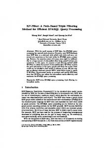
Figure 1: Example of interpolation in the 1dimensional case. Two possible positions are considered for the edge to be reconstructed. By evaluating the differences a - b and c - d it is possible to estimate the edge position from the low resolution image. Fig. 1 shows the effect of the position of the edge in the high-resolution data (A) and on the lowpass filtered and decimated data (C). Given the four consecutive pixels U , b, c, and d , an ideal interpolator should yield for the pixel II: (which lies between b and c) a value similar either t o the one of b (left) or to the one of c (right). Linear interpolation (D) fails to achieve this result. For the operator we propose, II: is computed as
x=,u~+(~-P)c, where
2. T H E ALGORITHM
p=
The interpolation is performed evaluating a nonlinear mean ol the pixels adjacent to the pixel 2 to be interpolated. Let us consider the one-dimensional case for simplicity.
0-7803-3258-X/96/$5.000 1996 IEEE
+
k l c - d)2 1 k ( ( u - b)2 ( c - cI)~) 2 '
-'
+
I
'
+
IC is a user defined parameter which controls the operator: for L = 0 a linear interpolation is obtained, while positive values for k yield the desired edge sensitivity.
711
When the edge is midway between b and c, a-b = c - d , SO that p = 0.5 and x = ( b + c ) / 2 , and the filter behaves as a linear one. When, in turn, the edge is asymmetrically located, the evaluated differences are no longer equal; for example, if the edge is closer to c (left column in the figure), then a - b < c - d , so that p > 0.5 and x N b. The proposed operator, being nonlinear, is capable of introducing frequencies between ~ / and 2 T , which have been lost during the lowpass/decimation process. This, of course, does not apply t o high frequency oscillations (not very common in natural images), but to the higher-order harmonics of the steps present in the original signal. In the following, some experiments with synthetic data are discussed. In Fig. 2a, a 128-element square wave (period 20) is considered. It is prefiltered with a gaussian lowpass filter (CT = 1, window length 5) and downsampled by a factor of 2. In the figure, the modulus of the D F T is shown for the original signal, our nonlinear interpolation, and the upsampled signal. The upsampled signal has been considered in order to show the frequency components of the mirror signal. In this case, the task of the interpolator is quite simple because the high frequencies of the mirror signal coincide with those of the original one. In Fig. 2b, a rectangular wave is considered which does not have constant period, so that its spectrum is more irregular. The nonlinear operator is able to reconstruct some of the harmonics of the original signal. It has t o be noticed that these frequencies are different from those of the mirror signal. The same comparison is reported in Fig. 3 for a horizontal line of the image ‘Lenna’. Also in this case, a good amount of high frequency components (which do not correspond t o those of the mirror signal) has been reintroduced by the proposed interpolator.
I 05
1
15
2
25
3
1
15
2
25
3
- - nonlinear inte
05
Figure 2: Complex modulus of the interpolated signal, in case of (a) a train of square waves; (b) a train of edges.
2.1. The two-dimensional case
The extension t o the two-dimensional case is described with reference to Fig. 4. Pixel 2 is interpolated using the one-dimensional filter applied on the mask shown in the left figure; similar considerations apply t o pixel y (center figure). Pixels of type x are dealt with after the other ones. For these, the proposed one-dimensional operator is applied t o the two masks shown in the right figure, using already interpolated pixels, and the mean value is assigned to 2.
Although very simple, this solution accurately reconstructs edges and allows us to avoid the evaluation of the edge direction. In fact, the proposed onedimensional operator correctly interpolates an edge when its mask is either parallel t o it or orthogonal t o it. This
7 12
may be easily seen for vertical or horizontal edges. Let us consider, for example, a vertical edge. When using the horizontal mask we reduce t o the already discussed one-dimensional case; the vertical mask, in turn, is parallel t o the edge so that the interpolation is trivial (and would be correct even with a linear filter). To understand the behaviour of the system with diagonal edges, let us refer t o Fig. 5. For each orientation (i.e., 45 and 135 degrees), four possible positions of the edge may be considered, two above the diagonal and two below it. We shall consider the former ones (the latter ones may be studied similarly); for each position, the edge is shown before (left) and after (right) the lowpass filtering. In the first case (Fig. 5a), pixels x and y will be reconstructed as very light grey using a horizontal and a vertical mask, respectively; in fact, with reference t o the right figure, there are two pixels with
I
I
0
0.5
1
1.5
2
2.5
3
Figure 3: Complex modulus for a horizontal line of the image ‘Lenna’.
Figure 4: Extension of the proposed algorithm to the two-dimensional case; o are the pixels of the decimated image. Left: pixel 2 is interpolated using the onedimensional proposed filter applied on the mask shown. Center: similar considerations apply to pixel y. Right: pixel z is obtained by the mean of the output of two one-dimensional filters of the type proposed, on the masks shown, using already interpolated pixels. Figure 5: Behavior of the proposed interpolator with diagonal edges (see text). For each of the two edge positions, (a) and (b), the edge is shown before (left) and after (right) the lowpass filtering.
the same grey level (white, in this case) from one side of the edge, and two pixels with different grey level (dark grey and black) to the other side. To interpolate pixel z , the vertical mask will give a very dark grey pixel because there are two (equally) black pixels at one side of the edge; also the horizontal mask will give a very dark grey pixel, for the same reason. It may be concluded that all the three interpolated pixels take values very similar t o those of the original data. The two masks that can be used for pixel z give essentially the same output; to cope with possible real image details, however, it is reasonable to take z as the mean value of the outputs of the two masks. It should be noted that a linear interpolator would yield a smoother transition:
x and y would be darker, while z would be lighter. The same conclusions can be drawn also for the second edge position considered in Fig. 5b. 3. EXPERIMENTAL RESULTS
Experimental results on both synthetic and real world images confirm the improvement of subjective image quality with respect to classical linear interpolators. As an example, a detail of the image ’Lenna’ is con-
713
I
I
I 100
200
300
400
500
600
700
variance threshold
Figure 7: PSNR (evaluated in the detail areas) versus variance threshold 8 for the proposed interpolator, a linear one and a cubic one. image. In order to evaluate the performance of the interpolation in the detail areas, we follow an approach similar to the one proposed in [3]. First, we label each pixel of the original image as a detail pixel if the local variance in its neighbourhood is above a given threshold 8. Then, the PSNR of the interpolated image is evaluated only for these detail pixels. The results are shown in Fig. 7 for various values of 8,for the part of image “Lenna” shown in Fig.6. It may be seen that with 8 increasing, i.e. when restricting our attention to smaller areas with higher variance, our interpolator significantly outperforms the others.
’ reconstructed by ng cubic convolu-
12 image has been lowpass filtered with a gaussian filter, decimated, and interpolated with our operator and with cubic convolution [a]. By inspection of the reconstructed images it may be seen that the edges (in particular, the border of the hat and the eye) are reconstructed more sharply by our operator. Also an objective measure of the interpolation error shows the good performances of the proposed approach: for our interpolator, a linear interpolator, and the cubic one, the PSNR’s are 30.82, 29.94, and 30.63 for the whole “Lenna” , respectively, and 28.94, 27.65, and 28.48 dB, respectively, for the detail shown in Fig. 6. The increment in the PSNR with respect t o the cubic interpolator is not very high; however, it has to be noted that the proposed algorithm is more accurate in the reconstruction of the details, which are very significant from a subjective point of view but which are generally represented by a minority of pixels in the
4. ACKNOWLEDGEMENTS This work has been partially supported by the European ESPRIT LTR Project # 20229 “NOBLESSE”. 5. REFERENCES
S. Lim, Two-dzmenszonal szgnal and zmage processzng. London: Prentice-Hall, Inc., 1990.
[l] J .
[a]
R. G. Keys, “Cubic convolution interpolation for digital image processing,” IEEE Trans. Acoust., Speech, Szgnal Processzng, vol. ASSP-29, no. 6, pp. 1153-1160, 1981.
[3] G. Ramponi, N. Strobel, S. E(. Mitra, T.-H. Yu, “Nonlinear unsharp masking methods for image contrast enhancement,” Journal of Electronzc Imagzng, 1996, t o appear.
714