Feb 9, 2012 - H ¨OLDERIAN REGULARITY-BASED IMAGE INTERPOLATION. Jacques Levy-Vehel. Pierrick Legrand. COMPLEX Team, INRIA Rocquencourt ...
Author manuscript, published in "ICASSP 06, International Conference on Acoustics, Speech, and Signal Processing, Toulouse : France (2006)" DOI : 10.1109/ICASSP.2006.1660788
¨ HOLDERIAN REGULARITY-BASED IMAGE INTERPOLATION Jacques Levy-Vehel
Pierrick Legrand
hal-00297218, version 1 - 9 Feb 2012
COMPLEX Team, INRIA Rocquencourt, 78153 Le Chesnay Cedex, France ABSTRACT We consider the problem of interpolating a signal in IRd known at a given resolution. In our approach, the signal is assumed to belong to a given (large) class of signals. This class is characterized by local regularity constraints, that can be described by a certain inter-scale behaviour of their wavelet coefficients. These constraints allow to predict the scale n coefficients from the ones at lower scales. We investigate some properties of this interpolation scheme. In particular, we give the H¨older regularity of the refined signal, and present some asymptotic properties of the method. Finally, numerical experiments are presented. Both the theoretical and numerical results show that our regularity-based scheme allows to obtain good quality interpolated images. 1. INTRODUCTION AND BACKGROUND A ubiquitous problem in signal and image processing is to obtain data sampled with the best possible resolution. At the acquisition step, the resolution is limited by various factors such as the physical properties of the captors or the cost. It is therefore desirable to seek methods which would allow to increase the resolution after acquisition. This is useful for instance in medical imaging or target recognition. At first sight, this might appear hopeless, since one cannot ”invent” information which has not been recorded. However, there are a number of situations of practical interest where this can be done. A first class of such situations is when several low resolution overlapping signals are available. This occurs in video sequences, radar imaging or MRI. Interpolation (also called superresolution in this context) is then the process of combining these multiple low resolution signals into a high resolution one. This is not the frame we shall consider here. In more general situations, a single signal is available for interpolation. Compared with the case above, one needs to supplement the data brought by the low resolution signal by a richer a priori information. Several methods have been explored, which may be roughly split into two types: In the first, ”class-based” one, the signal is assumed to belong to some class, with conditions expressed mainly in the time or frequency domain. Such classes include band-limited or timelimited signals, positive and/or sparse signals, and smooths ness classes such as C n or Besov spaces Bp,q . This puts
constraints on the interpolation, which is usually obtained as the minimum of a two-terms cost-function: The first term ensures that the reconstructed high resolution image is compatible with the observed low resolution one. The second term corresponds to the a priori smoothness information. Works following this approach include [1, 2, 3, 4, 5, 6, 7]. The second type of approach, which could be called ”contextual”, has been proposed in recent papers originating from several communities (computer vision, computer graphics, AI) [8, 9, 10]. It originates from the observation that most classbased methods results in overly smooth images at higher interpolation rates (i.e. larger than 4). Contextual methods try to overcome this problem by using a ”local learning” technique: Basically, the system is given some information about the local features in a given class of signals (a database). It then uses this information to compute a high resolution signal by comparing the local features of the signal to be processed with the ones of the signals in the database. The assumption is that neighbourhoods in the images of the database that are similar at resolutions n, n − 1, . . . , n − i, should remain so at the ”superresolution” n + 1. The methods then proceed by finding, for any neighbourhood in the image to be processed, similar neighbourhoods in the database, and then interpolating on the basis on the known high resolution versions of the database neighbourhoods. A number of problems remain with most techniques developed so far: While the interpolated image is usually too smooth, it also occur sometimes that on the contrary too many details are added, in particular in smooth regions. In addition, the creation of details is not well controlled, so that one can neither predict how the high resolution image will look like, nor the theoretical properties of the interpolation scheme. Let us now explain in informal terms how our method works. Broadly speaking, our main motivation is to find a way to interpolate in such a way that smooth regions as well as irregular ones (i.e. sharp edges or textures) remain so after zooming. We interpret this as a constraint on the the local regularity: The interpolation method should preserve the local regularity. The next step is to define an index of local regularity which is both a reasonable measure of the perceived regularity and mathematically/computationally tractable. In that view, we use a notion of H¨older exponent. H¨older exponents have been shown to correspond to an intuitive notion
hal-00297218, version 1 - 9 Feb 2012
of regularity in both images and 1D signals [11]. In order to control the interpolation and to obtain a simple implementation, we need to make some assumptions on the signal, to the effect that (a) this H¨older exponent can be easily estimated from wavelet coefficients (b) the H¨older exponent allows to predict the finer scales coefficients. Technically, this requires that the signal is not oscillatory (see section 2). This scheme allows to control both the reconstruction error and the regularity of the interpolated signal (this regularity does not depend on assumptions on the original signal). This regularity in turn controls the visual appearance of the added information, i.e. the (local) high frequency content. To get an intuitive understanding of the method, it is useful to recast this in terms of wavelet coefficients: Let X denoted the input signal and let dj,k be its wavelet coefficients, where, as usual, j corresponds to scale and k to location. Roughly speaking, if a signal has regularity α at point t, then its wavelet coefficient dj,k(j,t) ”above” t are bounded by C2−jα for some constant C: ∀j = 1 . . . n, |dj,k(j,t) | ≤ C2−jα . As said above, α correspond to an intuitive notion of regularity: A large α translates in a smooth signal, while α ∈ (0, 1) means that the signal is continuous and non differentiable at t. If the signal is discontinuous at t but bounded, then α = 0. Now if we are willing to preserve the regularity, we should prescribe the wavelet coefficient above t at the superresolved scale n + 1 in such a way that |dn+1,k(n+1,t) | ≤ C2−(n+1)α . For concreteness, let us explain schematically how our method would act in two simple situations: On a uniform region, all the wavelet coefficients are close to zero. The bound on the wavelet coefficients then holds with arbitrarily large α, since 0 ≤ C2−jα for all α > 0. As a consequence, the predicted coefficient dn+1,k will be zero, since it must satisfy the same inequality: The smooth region will remain smooth, because no detail will be added. On the other hand, above a step edge, the wavelet coefficients dj,k do not decay in scale. This imply that α = 0. The predicted coefficient dn+1,k will then be of the same order as dn,k . As a consequence, the local regularity of the interpolated image will be again equal to 0 at this point, and the edge will not be blurred. We describe the interpolation procedure in the next section. Section 3 highlights some theoretical features of the method related to asymptotic regularity properties of the interpolated signal and bounds on the reconstruction error. Finally, section 4 displays some numerical experiments. 2. THE METHOD Let X denote the original signal, and Xn = (xn1 , . . . xn2n ) its regular sampling over the 2n points (tn1 , . . . tn2n ). Let ψ denote a wavelet such that the set {ψj,k }j,k forms an orthonormal basis of L2 . Let dj,k be the wavelet coefficients of X. For k = 1 . . . 2n , we consider the point t = tnk and the wavelet coefficients dj,k(j,t) which are located ”above” it (ie k(j, t) = ⌊(t + 1)2j+1−n ⌋). Let αn (t) denote the slope of
the liminf regression of the vector (log(d1,k(1,t) , . . . dn,k(n,t) ) versus (−1, . . . , −n). See [12] for an account on liminf regressions. When n tends log dn,k(n,t) to infinity, αn (t) tends to liminf . This number has −n been considered in the literature [13] under the name of weak scaling exponent, denoted βw . It is a measure of the local regularity in the following sense. The weak scaling exponent of the signal X at t0 is defined as: βw = sup{s : ∃n, X (−n) ∈ Cts+n }. 0 where X (−l) denotes a primitive of order l of X and Cts0 is the usual pointwise H¨older space at t0 . When the local H¨older exponent αl and the pointwise H¨older exponent αp of X at t coincide, then βw is also equal to their common value. See [14] for more on this topic. In the following we will always assume that this is the case. In other words, we consider that our signals belong to the class S defined as follows: S = {X ∈ L2 (IR), ∀t ∈ IR, αp (t) = αl (t)} The class S may appear somewhat abstract to the reader. ∞ Here are a few clues. P S containsγnall C signals and all signals of the type n∈IN |t − tn | , with tn ∈ IR, γn ∈ IR+ . Many everywhere irregular signals are also in S, such as nowhere differentiable Weierstrass function Pthe continuous −nh n 2 sin(2 t), h ∈ (0, 1). On the other hand, ”chirp” n∈IN γ signals as |t| sin(1/|t|β ), γ > 0, β > 0 do not belong to S. The easiest way to picture elements in S is maybe through their wavelet transform: At each point t, the ”largest” coefficients are located above t in the following sense. Take any sequence dj,k of coefficients such that k2−j tends to t. Then, if X belongs to S, liminf j→∞
log |dj,k(j,t) | log |dj,k | ≥ liminf j→∞ −j −j
(1)
For a general continuous signal (i.e. a signal not in S), the H¨older regularity at t may always be evaluated from the decay of all the wavelet coefficients dj,k such that k2−j tends to t (i.e. from liminf such as above). When the signal is in S, inequality (1) implies that we may restrict our attention to the ones above t. Such signals are called ”non-oscillatory” in the literature. To perform the interpolation, we compute above each point t the regression of the wavelet coefficients vs scale. The parameters of the regression allow to build the extrapolated coefficient. These coefficients in turn determine the ”superresolved” signal.
3. REGULARITY AND ASYMPTOTIC PROPERTIES We give two properties of the regularity-based interpolation. ˜ n+m the signal See [15] for more results and proofs. Let X ˜ after �m interpolations, βn,k the slope of the regression and � e log Kn+1,k the ordinate in zero. 2
Proposition 1 If X ∈ C α then, whatever the number m of added scales: ˜ n+m k22 ≤ kX −X
ˆn c2 1 K ˆ 2−2βn n 2−2αn + ˆ 2α 2 β n 2 2 −1 2 −1
b n+1 , βbn ) such as: With (K b n+1 2−2j(βˆn + 12 ) = K
max
e n+1,k ,β˜n,k ) (K
h
e n+1,k 2−2j(β˜n,k + 12 ) K
i
Proposition 2 Let X belong to S, and assume X ∈ C α . Then, ∀ε > 0, ∃N : ˜ n+m ||2 = O(2−(n+m)(α−ε) ) n > N ⇒ ||X − X
hal-00297218, version 1 - 9 Feb 2012
In addition, ˜ n+m ||B s = O(2−(n+m)(α−s−ε) ) for all s < α − ε. ||X − X p,q 4. NUMERICAL EXPERIMENTS We present results of the regularity-based interpolation on two images. The first one is the well-known Lena image, the second is a scene containing a Japonese door (toryi ). Both original images are 128x128 pixels and are shown on figure 1. Figure 2 displays a comparison between four-times bicubic and regularity-based interpolations on a detail of Lena. Figure 3 presents eight-times bicubic and regularity-based interpolations on a detail of the door image.
Fig. 1. Original Lena and Door images, 128x128 pixels
5. REFERENCES [1] A. Papoulis, “A new algorithm in spectral analysis and bandlimited extrapolation,” IEEE Tr. Circuits Syst., vol. 22, no. 9, pp. 735–742, 1975.
Fig. 2. 4 times interpolation on a detail of Lena: bicubic (up), regularity-based (bottom)
[2] M.I. Sezan and H. Stark, “Image restoration by the method of convex projection: Part II - applications and numerical results,” IEEE Tr. Med. Imag., vol. 1, no. 2, pp. 95–101, 1982. [3] D. Slepian and H.O. Pollak, “Prolate spheriodal functions, Fourier analysis and uncertainty - I,” Bell Syst. Tech. J., vol. 40 (1), pp. 43–63, 1961. [4] D.C. Youla and H. Webb, “Image restoration by the method of convex projections: Part I - theory,” IEEE Tr. Med. Imag., vol. 1 (2), pp. 81–94, 1982. [5] P.J.S.G. Ferreira, “Noniterative and faster iterative for interpolation and extrapolation,” IEEE Tr. Sig. Proc., vol. 42, pp. 3278–3282, 1994. [6] D. Donoho, “De-noising by soft-thresholding,” IEEE Trans. Inf. Theory 41, pp. 613–627, 1994.
hal-00297218, version 1 - 9 Feb 2012
[7] K.-L Kueh, T. Olson, D. Rockmore, and K.-S Tan, “Non-linear Approximation Theory on Finite Group,” 1999. [8] F.M. Candocia and J.C. Principe, “Superresolutions of images based on local correlations,” IEEE Tr. Neural Networks, vol. 10, no. 2, pp. 372–380, March 1999. [9] S. Baker and T. Kanade, “Super-resolution: Reconstruction of Recognition,” Proc. of IEEE-Eurasip Workshop on Nonlinear Signal and Image Processing, pp. 349– 385, 2001. [10] W.T. Freeman, T.R. Jones, and E.C. Pazstor, “ExampleBased Super-Resolution,” MERL Tech. Rep., vol. 30, 2001. [11] J. Levy Vehel, “Fractal Approaches in Signal Processing,” Fractals, vol. 4, pp. 755–775, 1995. [12] J. Levy Vehel and P. Legrand, “Signal and Image Processing with FracLab,” FRACTAL 2004, Complexity and Fractals in Nature, 8th International Multidisciplinary Conference, Vancouver, 4-7 April 2004. [13] Y. Meyer, “Wavelets, Vibrations and Scalings,” American Mathematical Society, CRM Monograph Series, vol. 9, 1997. [14] J. Levy Vehel and S. Seuret, “The 2-microlocal Formalism,” Fractal geometry and Applications: A jubilee of Benoit Mandelbrot, Proc. Sympos. Pure Math., vol. 722, pp. 153–215, 2004. [15] P. Legrand, Debruitage et interpolation par analyse de la regularit´e Holderienne. Application l’analyse du frottement pneumatique/chauss´ee., Ph.D. thesis, 2004.
Fig. 3. 8 times bicubic (up) and regularity-based (bottom) interpolations on Door image (detail).