support vector machine classification of object-based data for crop ...

International Archives of the Photogrammetry, Remote Sensing and Spatial Information Sciences, Volume XXXIX-B7, 2012 XXII ISPRS Congress, 25 August – 01 September 2012, Melbourne, Australia

SUPPORT VECTOR MACHINE CLASSIFICATION OF OBJECT-BASED DATA FOR CROP MAPPING, USING MULTI-TEMPORAL LANDSAT IMAGERY R. Devadasa, *, R. J. Denhama and M. Pringlea a

Remote Sensing Centre, Ecosciences Percinct, GPO Box 2454, Brisbane, Queensland 4001, Australia – (rakhesh.devadas, robert.denham, matthew.pringle)@derm.qld.gov.au VII/4: Methods for Land Cover Classification

KEY WORDS: object-based, classification, Landsat, crop, artificial_intelligence/SVM, multitemporal ABSTRACT: Crop mapping and time series analysis of agronomic cycles are critical for monitoring land use and land management practices, and analysing the issues of agro-environmental impacts and climate change. Multi-temporal Landsat data can be used to analyse decadal changes in cropping patterns at field level, owing to its medium spatial resolution and historical availability. This study attempts to develop robust remote sensing techniques, applicable across a large geographic extent, for state-wide mapping of cropping history in Queensland, Australia. In this context, traditional pixel-based classification was analysed in comparison with image object-based classification using advanced supervised machine-learning algorithms such as Support Vector Machine (SVM). For the Darling Downs region of southern Queensland we gathered a set of Landsat TM images from the 2010-2011 cropping season. Landsat data, along with the vegetation index images, were subjected to multiresolution segmentation to obtain polygon objects. Object-based methods enabled the analysis of aggregated sets of pixels, and exploited shape-related and textural variation, as well as spectral characteristics. SVM models were chosen after examining three shape-based parameters, twenty-three textural parameters and ten spectral parameters of the objects. We found that the object-based methods were superior to the pixel-based methods for classifying 4 major landuse/land cover classes, considering the complexities of within field spectral heterogeneity and spectral mixing. Comparative analysis clearly revealed that higher overall classification accuracy (95%) was observed in the object-based SVM compared with that of traditional pixel-based classification (89%) using maximum likelihood classifier (MLC). Object-based classification also resulted speckle-free images. Further, object-based SVM models were used to classify different broadacre crop types for summer and winter seasons. The influence of different shape, textural and spectral variables, and their weights on crop-mapping accuracy, was also examined. Temporal change in the spectral characteristics, specifically through vegetation indices derived from multi-temporal Landsat data, was found to be the most critical information that affects the accuracy of classification. However, use of these variables was constrained by the data availability and cloud cover. analysis of aggregated sets of pixels, and exploit shape-related and textural variation, as well as spectral characteristics (Baatz and Schäpe, 2000). In the classification process, all pixels in the entire objects are assigned to the same class, thus removing the problems of spectral variability and mixed pixels (PeñaBarragán et al., 2011).

1. INTRODUCTION Land management practices have significant impacts on the condition of land and water and the profitability and sustainability of agriculture. Crop mapping and time series analysis of agronomic cycles are critical for monitoring landuse and land management practices, and analysing the issues of agro-environmental impacts and climate change.

Numerous classification algorithms have been developed since acquisition of the first Landsat image in early 1970s (Townshend, 1992). Maximum likelihood classifier (MLC), a parametric classifier, is one of the most widely used classifiers (Dixon and Candade, 2007; Hansen et al., 1996). The support vector machine (SVM) represents a group of theoretically superior non-parametric machine learning algorithms. There is no assumption made on the distribution of underlying data (Boser et al., 1992; Vapnik, 1979; Vapnik, 1998). The SVM employs optimization algorithms to locate the optimal boundaries between classes (Huang et al., 2002) and can be successfully applied to the problems of image classification with large input dimensionality. SVMs are particularly appealing in the remote sensing field due to their ability to generalize well even with limited training samples, a common limitation for remote sensing applications (Mountrakis et al., 2011).

Developments in remote sensing techniques offer a powerful and cost effective means for land use/land cover mapping, by virtue of their synoptic coverage and their ability to collect data at different spatial, spectral, radiometric and temporal resolutions. Multi-temporal Landsat data can be used to analyse decadal changes in cropping patterns at paddock level, owing to its medium spatial resolution and historical availability. Various investigations have demonstrated the benefits of crop mapping using remote sensing data (Congalton et al., 1998; Oetter et al., 2001; Ulaby et al., 1982). Utilisation of time series satellite data was proved to be essential for high accuracy of crop classification (Barbosa et al., 1996; Serra and Pons, 2008; Simonneaux et al., 2008). Object-based techniques have been increasingly implemented in remotely sensed image analysis to overcome problems due to pixel heterogeneity and crop variability within the field (Blaschke, 2010; Castillejo-González et al., 2009; PeñaBarragán et al., 2011). Object-based image analysis segments the image and constructs a hierarchical network of homogeneous objects. Object-based methods enable the

In this context, this study attempts to develop robust SVMbased techniques for classification of object-based data generated from multi-temporal Landsat images. Operational application of these techniques across a large geographic extent,

185

XXII Congress of ISPRS International Archives of the Photogrammetry, Remote Sensing and Spatial Information Sciences, Volume XXXIX-B7, 2012 XXII ISPRS Congress, 25 August – 01 September 2012, Melbourne, Australia

A cloud-free image composite was generated by selecting a primary image and replacing cloud-affected pixels with cloudfree pixels from images as close in time to the primary image as possible. For the summer growing season, an image acquired in February was selected as the primary image, whereas an image acquired in September was chosen as the primary image for the winter growing season. 2.4 Segmentation

for state-wide mapping of cropping history in Queensland, Australia, is also investigated. 2. METHODS 2.1 Study area Queensland is the 2nd largest state of Australia, covering over 1.7 million square kilometres, and a broad range of climate zones, topography, vegetation communities, geological landforms and soils. The study focussed on a Landsat scene area (path 90 and row 79) covering about 352,456 hectares (Figure 1).

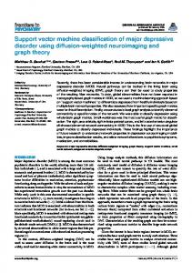
The multiresolution segmentation algorithm was applied to Landsat image composites, to partition the image into objects, using eCognition Developer 8.64.0 (Trimble, München, Germany) (Figure 2). The multiresolution segmentation algorithm is a bottom-up segmentation algorithm, based on a pairwise region-merging technique. This is an optimization procedure which, for a given number of image objects, minimizes the average heterogeneity and maximizes their respective homogeneity (Trimble, 2010).

Figure 2. Segmenation of Landat image using eCoginition. Yellow lines indicate segment delineation. The images is visualised as false colour composite by projecting near infrared, red and green bands as red, green and blue, respectively.

Figure 1. Location map of study area. Green areas indicate cropping regions for summer 2010. The growing season for summer crops is from December to April; the growing season for winter crops is from June to November. The study analysed satellite data for two crop seasons; summer 2010 (December 2010-April 2011) and winter 2011 (June 2011-November 2011). For summer 2010, 13 Landsat images and for winter 2011, 14 Landsat images were downloaded from USGS (http://glovis.usgs.gov/). 2.2 Pre-processing of Landsat data

The segmentation procedure starts with single image objects of one pixel and repeatedly merges them in several loops in pairs to larger units as long as an upper threshold of homogeneity is not exceeded locally. This homogeneity criterion is defined as a combination of spectral homogeneity and shape homogeneity. The ‘scale’ parameter influences this calculation, with higher values resulting in larger image objects, smaller values in smaller image objects (Trimble, 2010). Colour and shape (smoothness and compactness) parameters define the percentage that the spectral values and the shape of objects, respectively, will contribute to the homogeneity criterion (Castillejo-González et al., 2009). This study applied values 90, 0.7, 0.3, 0.5 and 0.5, for scale, colour, shape, smoothness and compactness, respectively, to generate meaningful image segments encompassing agricultural fields. 2.5 Support Vector Machine (SVM) classification

Landsat 5TM and Landsat 7ETM+ data have spatial resolution of 30m with a 16 day revisit period. The swath width is 185 km with 7 spectral bands in visible, near infrared, mid infrared and thermal infrared (NASA, 2011). Radiometrically calibrated and orthocorrected images were acquired from USGS and an empirical radiometric correction was then applied to reduce the combined effects of surface and atmospheric bidirectional reflectance distribution function (BRDF)(Danaher, 2002; de Vries et al., 2007). This method incorporates conversion from radiance to top-of-atmosphere reflectance with a modified version of the Walthall empirical BRDF model (Walthall et al., 1985), which was parameterised using pairs of overlapping ETM+ images. 2.3 Cloud masking and image compositing

Classification of the image objects obtained from the segmentation procedure was carried out using the SVM technique. In the first phase, the study attempted to classify the objects into four major classes: fallow, crop, pasture and woody vegetation. In the following phase, the potential of SVM to classify different crop types was examined.

Automated cloud detection and masking were carried out on each image using cloud-detection techniques developed at the Queensland Remote Sensing Centre (Goodwin et al., 2011). The approach locates anomalies in the reflectance time series (large differences in reflectance between cloud affected and predicted non-cloud affected observations) and incorporates region-growing filters to spatially map the extent of the cloud / cloud shadow

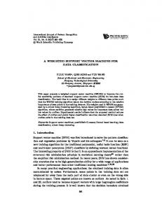
A SVM optimally separates the different classes of data by a hyperplane (Karatzoglou and Meyer, 2006; Kavzoglu and Colkesen, 2009; Vapnik, 1998). The points lying on the boundaries are called support vectors and the middle of the margin is the optimal separating hyperplane (Meyer, 2001; Mountrakis et al., 2011) (Figure 3).

186

XXII Congress of ISPRS International Archives of the Photogrammetry, Remote Sensing and Spatial Information Sciences, Volume XXXIX-B7, 2012 XXII ISPRS Congress, 25 August – 01 September 2012, Melbourne, Australia

Vegetation indices Normalised Difference Index 4-7  B4 − B7  NDI47 =    B4 + B7 

Normalized Difference Index 4-5  B4 − B5  NDI45 =    B4 + B5 

Enhanced Vegetation Index

(Huete et al., 2002)

B4 − B3   EVI = G   B4 + C1xB3 - C2xB1 + L 

G=2.5, C1=6, C2=7.5 and L=1 Modified Chlorophyll Absorption and Reflectance Index

Figure 3. Classification using support vectors and separating hyperplane (Meyer, 2001). Hollow and solid dots represent two classes in feature space.

 B4  MCARI = [(B4 − B3) − 0.2(B4 − B2 )]   B3 

Green Normalised Difference Vegetation Index

An optimum hyperplane is determined using a training dataset, and its generalization ability is verified using a validation dataset. Training vectors xi are projected into a higher dimensional space by the function φ . SVM finds a linear separating hyperplane with the maximal margin in this higher dimensional space. The methodology for SVM implementation are well described by Karatzoglou and Meyer (2006) and Kavzoglu and Colkesen (Kavzoglu and Colkesen, 2009). The study used a polynomial kernel and employed ‘one-against-one’ technique to allow multi-class classification. The SVM algorithm was implemented in R open-source software (Chang and Lin, 2001; Meyer, 2001) 2.6 Training data collection

 B4 − B2  GNDVI =    B4 + B2 

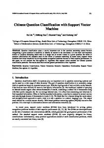
3. RESULTS AND DISCUSSION Ground reference data collected (Section 2.6) for crop seasons summer 2010 and winter 2011 were analysed in conjunction with the spatial data variables described in Section 2.7. Random forest variable importance analysis showed that the range of EVI was the most influential variable. Temporal signatures of average EVI values derived for different classes during the crop season of summer 2011 are illustrated in Figure 4. Areas of cropping consistently shows higher range of EVI values compared with bare soil or pasture, due to the spectral variations associated with the crop phenological changes during the crop season.

Three shape-based parameters, twenty-three textural parameters and ten spectral parameters of the objects were analysed to determine the appropriate set of input variables for the SVM model. A combination of random forest variable importance measures (Breiman, 2001; Liaw and Wiener, 2002) and repeated classification accuracy assessment procedure was carried out for model reduction and the selection of input variables. Based on this analysis, the following variables (Table 1) were chosen as input to SVM model.

0.8 0.7 0.6

Table 1. Spectral and textural input variables selected for SVM modelling Variable name and formula References Textural parameters Grey level co-occurrence matrix (GLCM) (Trimble, Entropy 2010)

Fallow Cotton Pasture Sorghum

EVI

0.5 0.4 0.3 0.2 0.1 0

N −1

Sep 2010

∑ Pij (− ln Pi, j)

Jan 2011

Feb 2011

Apr 2011

Figure 4. Temporal changes in mean EVI values for different classes during summer 2010 crop season derived from Landsat time series data

i , j =0

i is the row number of the image j is the column number Pi,j is the normalised value in the cell i,j Pi , j =

(Gitelson and Merzlyak, 1996)

Temporal spectral variables EVI-range (winter/summer crop season) EVI-minimum (winter/summer crop season) Other spectral variables Reflectance in Blue-Green (B1) Reflectance in Red (B3) Reflectance in Near Infrared (B4) Reflectance in Mid Infrared (B5) B indicates the band of Landsat data converted to exoatmospheric reflectance. eg. B4 means band 4 as shown in Landsat hand book (NASA, 2011).

Spatially diffuse training data sets covering the study area were collected for two crop seasons, summer 2010 and winter 2011. A global positioning system and a laptop computer were used to record the dominant vegetation species at particular roadside locations. Nearly 50% of the data points collected for each crop season was utilised for SVM modelling and remaining data sets were used for validation purposes. 2.7 Selection of input variables

GLCM Entropy =

(Daughtry et al., 2000)

Accuracy assessment clearly demonstrated the potential of SVM techniques for classification of the major classes (fallow, crop, pasture and woody). Overall classification accuracy for summer 2010 was 87% (k = 0.73)(Table 2) while that of winter 2011 was 93% (k = 0.9) ( ).

V

i, j N −1

∑V

i, j

i , j =1

Vi, j is the value in the cell i, j of the matrix N is the number or rows or columns

187

XXII Congress of ISPRS International Archives of the Photogrammetry, Remote Sensing and Spatial Information Sciences, Volume XXXIX-B7, 2012 XXII ISPRS Congress, 25 August – 01 September 2012, Melbourne, Australia

crop types. For summer, cotton and sorghum were considered as the major crops and crops like sunflower, mung beans, millets and fodder crops were grouped into a class called other crops. The SVM model generated classified the image into these broadacre crop types (Figure 6) with an overall accuracy of 78% (k = 0.7) (Table 4).

Table 2. Accuracy assessment of summer 2010 classification (major classes only) Classes

Classified

Fallow Crop Fallow 68 7 Crop 30 369 Pasture 1 0 Woody 0 0 Total 99 376 Overall accuracy = 87% Kappa coefficient (k) = 0.73

Reference Pasture 1 23 14 0 38

Woody 0 6 1 38 45

Total 76 428 16 38 558

Lower classification accuracy in the case of summer data could be attributed mainly to two reasons. During summer, there was more classification error between crop and pasture. High amount of rainfall during the summer growing season causes a significant increase in vegetative growth in pasture areas and this in turn could make it difficult to distinguish these areas from cropping, spectrally. The second reason could be the noticeably higher cloud cover during the summer. It may be noted that EVI range is observed to be the most important input variable for SVM modelling and cloud-affected pixels could decrease the number pixels available for EVI range estimation over the growing season. Further, a separate analysis, carried out by omitting training data sets over cloud-affected pixels, indicated the accuracy could be as high as 95 % (k = 0.9). The MLC was applied on the same dataset and the results clearly revealed that SVM techniques not only produced superior classification accuracy, but also generated a neater and speckle-free image (Figure 5).

Figure 6. Classification of broad acre crop types for summer 2010 and winter 2011 Table 4. Accuracy assessment of summer 2010 classification of crop types Reference Cotton Fallow Other crops Pasture Sorghum Woody Cotton 162 6 8 5 16 2 Fallow 1 72 4 1 2 0 Other crops 0 2 7 0 0 0 Pasture 0 2 2 20 0 1 Sorghum 19 17 23 12 132 1 Woody 0 0 0 0 0 41 Total 182 99 44 38 150 45 Overall accuracy = 78% Kappa coefficient (k) = 0.70

Classified

Classes

Total 199 80 9 25 204 41 558

Similarly, SVM models were generated for separating broadacre crop types for winter 2011 (Figure 6). Major crop types identified were barley and wheat. Crops like chick pea, and fodder were grouped into other crops. Winter crop type classification accuracy was again found to be slightly higher (79%, k = 0.73) than that of summer (Table 5). Table 5. Accuracy assessment of winter 2011 classification of crop types

Table 3. Accuracy assessment of winter 2011 classification (major classes only)

Classes

Classes

Classified

Fallow Crop Fallow 70 0 Crop 0 244 Pasture 0 1 Woody 0 1 Total 70 246 Overall accuracy = 93% Kappa coefficient (k) = 0.90

Reference Pasture 0 4 158 0 184

Woody 0 4 8 78 90

Total 70 274 167 79 590

Classified

Figure 5. Comparison of Support Vector Machines and Maximum Likelihood Classified images

Reference Barley Fallow Other crops Pasture Wheat Barley 14 0 3 0 2 Fallow 0 70 0 0 0 Other crops 6 0 11 0 3 Pasture 3 0 11 178 7 Wheat 30 0 27 6 134 Woody 0 0 2 0 2 Total 50 70 54 184 0 Overall accuracy = 79% Kappa coefficient (k) = 0.73

Woody 0 0 0 12 0 78 90

Developing operational methods for the assessment of crop distribution is crucial for the effective implementation of agricultural policies. For example, the State Government of Queensland, Australia, passed the Strategic Cropping Land (SCL) Bill in December 2011 to protect land that is highly suitable for cropping, manage the impacts of development on

This project aims to develop operational methods for crop type classification for Queensland. In pursuit of this, a preliminary investigation was attempted to classify broadacre crop types for both crop seasons. For summer 2010, the crop class mapped in the first phase (Table 2 and ) was further classified to different

188

Total 20 70 20 211 197 80 598

XXII Congress of ISPRS International Archives of the Photogrammetry, Remote Sensing and Spatial Information Sciences, Volume XXXIX-B7, 2012 XXII ISPRS Congress, 25 August – 01 September 2012, Melbourne, Australia

that land and preserve the productive capacity of that land for future generations (Figure 7). (See http://www.derm.qld.gov.au/land/planning/strategiccropping/index.html ).

4. CONCLUSIONS Results of this study demonstrated the distinctive advantage of object-based methods over pixel-based methods, considering the complexities of within-field spectral heterogeneity and spectral mixing. This is well supported by several other studies (Castillejo-González et al., 2009; Peña-Barragán et al., 2011). This investigation further combined the superiority of objectbased data with a powerful non-parametric SVM classifier (Boser et al., 1992; Dixon and Candade, 2007; Huang et al., 2002) to perform automated large-area broadacre crop mapping. Comparative analysis clearly revealed that substantially higher overall classification accuracy (95%) was observed with the object-based SVM, compared with that of traditional pixelbased classification (89%). Object-based classification also resulted in neater and speckle-free images. Further, objectbased SVM models were used to classify different broadacre crop types for summer and winter seasons. Influence of different shape, textural and spectral variables and their weights on crop-mapping accuracy was also examined. Temporal change in the spectral characteristics, specifically through vegetation indices derived from multi-temporal Landsat data, was found to be the most critical information that aftected the accuracy of classification using SVM models. However, use of these variables was constrained by the multi-temporal data availability and cloud cover. ACKNOWLEDGMENTS

Figure 7. Cropping areas detected by this study within the Strategic Cropping Land trigger map during summer 2011, as indicated by green patches in the map. Overlaid is the footprints of 35 Landsat scenes that cover the study area.

Authors wish to thank United States Geologic Survey (USGS) for providing Landsat images used for this study.

The legislation aims to restrict developmental activities on cropping areas, which have been cultivated at least three times between 1 January 1999 to 31 December 2010 and that meet on-ground assessment against the site level SCL criteria. This has generated a demand for automated large area crop classification.

REFERENCES Baatz, M., Schäpe, A., 2000. Multi-resolution segmentationAnoptimization approach for high quality multi-scale segmentation, in: Strbl, J. (Ed.), Angewandte Geographische Informationsverarbeitung XII. Beiträge zum AGIT-Symposium 2000. Karlsruhe, Herbert Wichmann Verlag, Salzburg, p. 12−23.

The trigger map indicates the location of potential SCL in Queensland and is based on soil, land and climate information. The SCL area extends to 42-million ha, which is almost onequarter of Queensland and requires 35 Landsat scenes to cover the entire area. SVM models were applied on these 35 sets of multi-temporal Landsat data to demarcate areas cropped during summer 2010 (Figure 7) and winter 2011 (Figure 8)

Barbosa, P.M., Casterad, M.A., Herrero, J., 1996. Performance of several Landsat 5 Thematic Mapper (TM) image classification methods for crop extent estimates in an irrigation district. International Journal of Remote Sensing, 17, pp. 36653674. Blaschke, T., 2010. Object based image analysis for remote sensing. ISPRS Journal of Photogrammetry and Remote Sensing, 65, pp. 2-16. Boser, B.E., Guyon, I., V, V., 1992. A training algorithm for optimal margin classiers, Fifth Annual Workshop on Computational Learning Theory. ACM Press, p. 144. Breiman, L., 2001. Random Forests. Machine Learning, 45, pp. 5-32. Castillejo-González, I.L., López-Granados, F., García-Ferrer, A., Peña-Barragán, J.M., Jurado-Expósito, M., de la Orden, M.S., González-Audicana, M., 2009. Object- and pixel-based analysis for mapping crops and their agro-environmental associated measures using QuickBird imagery. Computers and Electronics in Agriculture, 68, pp. 207-215.

Figure 8. Cropping areas detected by this study within the Strategic Cropping Land trigger map during winter 2011, as indicated by green patches in the map.

189

XXII Congress of ISPRS International Archives of the Photogrammetry, Remote Sensing and Spatial Information Sciences, Volume XXXIX-B7, 2012 XXII ISPRS Congress, 25 August – 01 September 2012, Melbourne, Australia

Chang, C.C., Lin, C.J., 2001. libsvm: A Library for Support Vector Machines. URL:http://www.csie.ntu.edu.tw/~cjlin/papers/libsvm.pdf.

Mountrakis, G., Im, J., Ogole, C., 2011. Support vector machines in remote sensing: A review. ISPRS Journal of Photogrammetry and Remote Sensing, 66, pp. 247-259.

Congalton, R.G., Balogh, M., Bell, C., Green, K., Milliken, J.A., Ottman, R., 1998. Mapping and monitoring agricultural crops and other land cover in the Lower Colorado River basin. Photogrammetric Engineering and Remote Sensing, 64, pp. 1107−1113.

NASA, 2011. Landsat 7 Science Data Users Handbook. NASA, URL:http://landsathandbook.gsfc.nasa.gov/pdfs/Landsat7_Han dbook.pdf, pp. 30-31. Oetter, D.R., Cohen, W.B., Berterretche, M., Maiersperger, T.K., Kennedy, R.E., 2001. Land cover mapping in an agricultural setting using multiseasonal Thematic Mapper data. Remote Sensing of Environment, 76, pp. 139−155.

Danaher, T., 2002. An empirical BRDF correction for Landsat TM and ETM+ imagery, 11th Australasian Remote Sensing and Photogrammetry Conference, Brisbane, Australia.

Peña-Barragán, J.M., Ngugi, M.K., Plant, R.E., Six, J., 2011. Object-based crop identification using multiple vegetation indices, textural features and crop phenology. Remote Sensing of Environment, 115, pp. 1301-1316.

Daughtry, C.S.T., Walthall, C.L., Kim, M.S., de Colstoun, E.B., McMurtrey Iii, J.E., 2000. Estimating Corn Leaf Chlorophyll Concentration from Leaf and Canopy Reflectance. Remote Sensing of Environment, 74, pp. 229-239.

Serra, P., Pons, X., 2008. Monitoring farmers' decisions on Mediterranean irrigated crops using satellite image time series. International Journal of Remote Sensing, 29, pp. 2293−2316.

de Vries, C., Danaher, T., Denham, R., Scarth, P., Phinn, S., 2007. An operational radiometric calibration procedure for the Landsat sensors based on pseudo-invariant target sites. Remote Sensing of Environment, 107, pp. 414-429.

Simonneaux, V., Duchemin, B., Helson, D., Er-Raki, S., Olioso, A., Chehbouni, A.G., 2008. The use of high-resolution image time series for crop classification and evapotranspiration estimate over an irrigated area in central Morocco. International Journal of Remote Sensing, 29, pp. 95-116.

Dixon, B., Candade, N., 2007. Multispectral landuse classification using neural networks and support vector machines: one or the other, or both? International Journal of Remote Sensing, 29, pp. 1185-1206.

Townshend, J.R.G., 1992. Land cover. International Journal of Remote Sensing, 13, pp. 1319-1328.

Gitelson, A.A., Merzlyak, M.N., 1996. Signature Analysis of Leaf Reflectance Spectra: Algorithm Development for Remote Sensing of Chlorophyll. Journal of Plant Physiology, 148, pp. 494-500.

Trimble, 2010. eCognition® Developer 8.64.0 Reference Book. Trimble Germany GmbH, Trappentreustr. 1, D-80339 München, Germany.

Goodwin, N., Collett, L., Denham, R., Tindall, D., 2011. Mapping long term fire history using a cloud affected time series of Landsat TM and ETM+ imagery for Queensland, Australia, 34th International Symposium on Remote Sensing of Environment, Sydney.

Ulaby, F.T., Li, R.Y., Shanmugan, K.S., 1982. Crop classification using airborne radar and Landsat data. IEEE Transactions on Geosciences and Remote Sensing, 20, pp. 518−528.

Hansen, M., Dubayah, R., Defries, R., 1996. Classification trees: an alternative to traditional land cover classifiers. International Journal of Remote Sensing, 17, pp. 1075-1081.

Vapnik, V., 1979. Estimation of Dependences Based on Empirical Data, Nauka, Moscow. (in Russian) English translation: Springer Verlag, New York, 1982.pp.5165-5184

Huang, C., Davis, L.S., Townshend, J.R.G., 2002. An assessment of support vector machines for land cover classification. International Journal of Remote Sensing, 23, pp. 725-749.

Vapnik, V., 1998. Statistical Learning Theory. Wiley, New York Walthall, G.L., Norman, J.M., Welles, J.M., Campbell, G., Blad, B.L., 1985. Simple equation to approximate the bidirectional reflectance from vegetative canopies and bare soil surfaces. Applied Optics, 24, pp. 383-387.

Huete, A., Didan, K., Miura, T., Rodriguez, E.P., Gao, X., Ferreira, L.G., 2002. Overview of the radiometric and biophysical performance of the MODIS vegetation indices. Remote Sensing of Environment, 83, pp. 195-213. Karatzoglou, A., Meyer, D., 2006. Support Vector Machines in R. Journal of Statistical Software, 15, pp. 1-28. Kavzoglu, T., Colkesen, I., 2009. A kernel functions analysis for support vector machines for land cover classification. International Journal of Applied Earth Observation and Geoinformation, 11, pp. 352-359. Liaw, A., Wiener, M., 2002. Classification and Regression by randomForest. R News: The Newsletter of the R Project, 2/3. Meyer, D., 2001. R News: The Newsletter of the R Project. 1, pp. 23-26.

190