quartets, weighting differences, distance correction, simulated evolution. method, minimum .... quartets (MQ; Dress et al. 1986). ..... Time warps, string edits and ...
A Simple Method to Improve the Reliability of Tree Reconstructions 1 Michael Sch6niger2 and Arndt von Haeseler3 Department
of Mathematics,
University
of Southern
California
The efficiencies of distance-matrix methods for correct tree reconstruction under a variety of substitution rates, transition-transversion biases, and different model trees were studied. If substitution rates are high and the ratio of transitions and transversions is large, even a Kimura two-parameter correction fails very often to reconstruct the model tree. We show that a combination of combinatorial weighting by Williams and Fitch and the Jukes-Cantor correction significantly increases the efficiency of tree-reconstruction methods, for a large fraction of evolutionary parameters. We explain why this approach is superior to any other weighting/correction scheme tested, as long as sequences are sufficiently long or substitution rates are sufficiently large. An approximate threshold for switching to a different weighting scheme is given.
Introduction As long as scientists have tried to reconstruct phylogenetic trees, they have debated how to weight differences (or, alternatively, similarities) between pairs of letters of the underlying alphabet. For nucleic acid sequences the alphabet consists of four letters, the nucleotides adenine (A), guanine (G), cytosine (C), and thymine (T) . The naive, but useful, approach to count the number of differences, the so-called Hamming metric on this alphabet, was put into question by the observation that transitions occur more frequently than transversions and that the transition-transversion bias is variable in different regions of the genome (Brown et al. 1982; Gojobori et al. 1982; Li et al. 1984; Hixson and Brown 1986). Therefore it is desirable to take into account those differences when a phylogenetic tree is calculated. Applying an inappropriate distance measure on the alphabet might lead to false conclusions about the phylogenetic relationships of the sequences under study (Sourdis and Nei 1988). Besides correctional methods for multiple hits (Jukes and Cantor 1969; Kimura 1980)) other proposals to improve the efficiency of tree-reconstruction methods have been made (Far-r-is 1969; Sankoff and Cedergren 1983; Williams and Fitch 1990). These methods assign different costs to various substitutional changes and/ or different positions in the sequences. Costs are estimated in an iterative procedure. Moreover, they require the repeated reconstruction of phylogenetic trees, in 1. Key words: phylogenetic tree, distance-matrix quartets, weighting differences, distance correction,
method, neighbor-joining simulated evolution.
method, minimum
misplaced
2. Present address: Theoretical Chemistry, Technical University Munich, Lichtenbergstrage 4, 8046 Garching,
Germany.
3. Present address and address for correspondence and reprints: Arndt Zoology, University of Munich, Luisenstral3e 14, 8000 Munich 2, Germany.
von Haeseler,
Institute
for
Mol. Biol. Evol. 10(2):471-483. 1993. 0 1993 by The University of Chicago. All rights reserved. 0737-4038/93/1002-0017$02.00 471
472
SchGniger and von Haeseler
order to obtain good cost estimates. Those reconstructions are computationally expensive. The change in efficiency of commonly used tree-reconstruction methods, if corrected evolutionary distances are calculated, has been analyzed in a series of papers (Blanken et al. 1982; Tateno et al. 1982; Tateno and Tajima 1986; Saitou and Nei 1987; Sourdis and Krimbas 1987; Saitou and Imanishi 1989; Jin and Nei 1990). Sequences were generated according to a model tree, and in some instances a transitiontransversion bias was introduced into the model. Both presence and absence of a molecular clock were investigated (i.e., constant and varying rates of substitution). In all cases the observed numbers of nucleotide differences (Hamming distances) were subsequently corrected by using either the Jukes-Cantor (JC) model or Kimura’s twoparameter (Km) model, the latter taking into account the transition-transversion bias between two sequences. It is hard to tell from the accumulated data which method is best, especially which correction gives the greatest efficiency in obtaining the modeled tree. However, as a rule of thumb, it seemed advisable to use the neighbor-joining (NJ) method (Saitou and Nei 1987) together with the Km correction. This was valid when the sequences under study did not evolve under a molecular clock. Most impressive are Jin and Nei’s ( 1990) results in that respect, when they investigate model trees (with four taxa) of extremely different rates of substitutions in the branches leading to two neighbor sequences. We tested NJ in combination with the Km correction on sequence data that evolved under a model tree with eight taxa, high substitution rates, and a strong transition-transversion bias, and we found that it performed rather poorly (see below). Therefore we suggest a new weighting and distance-correction scheme that permits one to handle these cases of evolutionary behavior as well. This is basically accomplished by assigning lower weights to more frequent, less informative substitutions and by assigning higher weights to rare, more informative ones. Our simulation tests divide into four natural subdivisions: ( 1) evolution of test sequences on a model tree, ( 2) weighting of character-state changes, ( 3) correction of observed differences for multiple changes, and (4) application of various methods to analyze the data. Methods Evolution
of Test Sequences
on a Model Tree
Our simulations were similar to those described by Sourdis and Nei ( 1988 ) . Each model contains four elements: (a) the topology of the tree, (b) the number of expected substitutions, per site, along each branch (rate), (c) the length of sequences, and (d) the fraction of substitutions that are transitions. We used the two model trees (T 1 and T2) depicted in figure 1. The topologies of the trees are identical. The parameters a and b along the branches of the trees are the expected numbers of nucleotide substitutions per site. An ancestral sequence of a given length I was generated using pseudorandom numbers by assuming equal base frequencies. In our simulations I was equal to either 500 or 1,000 nucleotides. This ancestral sequence evolved according to the branching pattern of the model tree. The actual numbers of substitutions along the branches were calculated by following a Poisson distribution with mean equal to the expected branch length. Three sets of parameters were studied for both trees: I, a = 0.01 and b = 0.07; II, a = 0.02 and b = 0.19; and III, a = 0.03 and b = 0.42. Note that the assignment of substitution rates along the branches of trees T, and
Distance Weighting and Correction
473
2
a
a
1 b
0.5a
-r
2
OSa
b
b
3
-i
f;b
I3
4
6 7 b
8
FIG. 1.-Model trees with expected substitution rates a and b. T,,Constant rate of substitution (i.e., CL). T2, Varying rate of substitution (i.e., NC).
T2 implies the existence of a stochastically constant molecular clock (CL) in T 1, whereas in T2 the nucleotide substitutions are varying [i.e., there is no molecular clock: (NC)]. NC-III has unequal rates as great as a factor of 14, along the branches leading to neighboring sequences. Parameter B defines the proportion of transitional changes among the total changes (Jin and Nei 1990). To obtain a transition-transversion bias we used a two-parameter model (Kimura 1980) with B = 0.8, i.e., a transitional change happened eight times (arbitrarily chosen) as frequently as did each of the two remaining transversional changes. We also studied a simple one-parameter model with B = 0.5, i.e., no transitiontransversion bias. The eight sequences produced as described above were subject to further analysis. Weighting of Character-State Changes The basic idea of weighting is to emphasize seldom observed, more informative substitutions and to suppress often occurring, less informative ones. The weighting of character-state changes in our simulation tests is either uniform (uf), existential (ex), or combinatorial (co). The latter ones were introduced for dynamically weighted maximum-parsimony procedures, by Williams and Fitch ( 1990). Distances were calculated as follows:
where a = (al, a2, . . . , al) and b = (bl, b2, . . . , bl) are sequences of length 1, ai, bi E ( A, G, C, T >, and t represents a symmetric weighting matrix with diagonal values tjj = 0. If t has off-diagonal values equal to 1, then the resulting distance Dab is the number of observed differences between a and b. Hence character-state changes are weighted uniformly (uf) . To compute a co weight matrix the number of occurrences w$’of differences of
474
SchGniger and von Haeseler
the type nucleotides i andj was counted for every pair of sequences these counts wtb for all possible pairs, we obtained
a and b. Summing
(2) The entries
oft are defined
as t(iJ)
= t(j,i)
=
(3)
L .fij*
If we define& as the number of alignment positions where nucleotides i andj are both observed and subsequently apply equation (3)) an ex matrix is calculated. To facilitate comparisons of distances derived from different weighting schemes, the weight matrices were normalized to an average off-diagonal matrix element of 1. Distances Dab can be viewed as weighted averages of numbers of transversions and numbers of transitions. Table 1 illustrates the procedure. Correction
for Multiple
Changes
Either multiple substitutions are uncorrected for (UC) or the JC or Km correction was applied. Correction JC (Jukes and Cantor 1969) is made by the following transformation:
d!icC’ = - 3/4 In (
Correction
Km (Kimura
(4)
I-bi33.
1980) is a more general scheme, using two parameters.
Table 1 Numerical Example for Different Weighting Schemes
trl
h WEIGHTING SCHEME AND A
NUCLEOTIDE
G
C
T
A
G
C
T
uf: A G C T ex: A G C T co: A G C T
...... ...... ...... ......
.. .... . . ...
...... ...... ...... ......
.. .... . .. ..
2
1 1
...... ...... ...... ......
. .... .. .. .
4
2 1
NOTE-The
0
1 0
1 1 0
1 I 2
0
0.6 0
1.2 1.2 0
1.2 1.2 0.6 0
2 I 3
0
0.42 0
0.84 1.67 0
0.84 1.67 0.56 0
three sample sequences (I = 9) used are AAGCTAAGC, AGATTCTGT, and AGGTTCTGG.
Distance Weighting and Correction
475
One preconceives a certain evolutionary model (i.e., that the rate of transitional nucleotide substitutions is different from that of transversional substitutions) and calculates corrected pair-wise distances from observed fractions of nucleotide sites showing transition (&,) and transversion (pii,) differences between the two sequences compared, according to dLt*) = - 1/2 ln[ ( 1-2pib-p&)m]
.
(5)
The three types of distances between two sequences, derived from uf, ex, or co weighting, were either left uncorrected for (uf/Uc, ex/Uc, and CO/UC) or had JC correction applied to them (uf/ JC, ex/ JC, and co / JC ) . To compute uf/ Km, ex / Km, and co/Km it was necessary to modify the definitions of pi,, and pib similarly to equation ( 1), using appropriate weights. If P:b
=
2Pib,
then Km correction is equivalent to JC correction. methods. served as data for tree-reconstruction Application
of Various
Methods
to Analyze
The nine possible distance
matrices
the Data
We evaluated the performance of two tree-building methods based on pairwise distances: ( 1) NJ (Saitou and Nei 1987) and (2) minimum number of misplaced quartets (MQ; Dress et al. 1986). The first was studied because in a variety of publications (e.g., Saitou and Nei 1987; Sourdis and Nei 1988; Saitou and Imanishi 1989; Jin and Nei 1990) NJ was shown to be very efficient in comparison with other commonly used tree-building methods. While NJ is a clustering method, MQ belongs to the class of tree-building methods that optimize an objective function on the set of tree topologies. In this case the tree with a minimal number of misplaced quartets is looked for (see Bandelt and Dress 1986; Dress et al. 1986). Results Constant
Rate of Nucleotide
Substitution
(i.e., CL)
We show in tables 2 and 3 the percentages PC of correctly reconstructed trees under a molecular clock; these two assume a transition-transversion bias of B = 0.3 and B = 0.8, respectively. Only the empirical probability of obtaining the correct unrooted tree was studied, because Sourdis and Nei ( 1988) observed a strong correlation between P, and the average topological distance from the model tree. However, a more detailed analysis of the distributions of topological deviations would yield more reliable criteria for comparing the efficiencies of various methods used (Tateno et al. 1982). The tree-reconstruction methods NJ and MQ yield more or less the same results, independent of the weighting/correction scheme. As already observed ( Saitou and Nei 1987; Sourdis and Nei 1988), the probability of reconstructing the model tree increases when substitution rates decrease or when the sequence length increases. This result does not depend on the transition-transversion bias, the weighting scheme, or the method. Both tree-reconstruction methods perform generally better when the sequences evolved under model B = 0.3 (compare table 2 with table 3). As long as the substitution
476
Schijniger
and von Haeseler
Table 2 Percentage P, of Correctly Inferred Reconstructed Trees, by Method, for CL Evolution (fig. 1, T1) and without Transition-Transversion Bias (B = 0.3) I: a/b = 0.01/0.07 WEIGHTING/CORRECTION SCHEME
I= 500
1 = 1,000
II: a/b = 0.02/0.19 1= 500
I = 1,000
III: a/b = 0.03/0.42 I = 500
I = 1,000
NJ: Ufi UC
JC Km ex: UC JC Km co: UC JC Km MQ:
.
. . . .
. ... .
71.5 70.3 70.5
95.3 94.9 94.7
53.3 51.3 52.0
87.2 86.7 86.8
9.1 8.4 8.2
40.6 38.1 38.3
... .....
. .. ....
70.7 70.3 70.3
95.1 94.5 94.6
53.0 51.7 51.8
87.3 86.7 86.6
9.2 8.2 8.2
40.9 38.7 38.9
. .. . ..
. ....
70.5 69.7 69.7
94.7 94.4 94.4
53.7 51.6 51.9
87.2 86.3 86.3
9.0 8.4 8.4
40.7 37.5 38.0
... . ..
....
68.9 66.6 67.7
93.7 93.0 93.4
51.8 49.7 49.4
84.8 83.4 83.8
7.3 7.2 6.5
37.6 35.2 36.1
.. ..
. . .. . ..
66.3 64.8 65.2
93.5 93.3 93.2
49.5 47.8 48.3
84.3 83.7 83.7
7.4 7.0 6.5
37.2 35.4 35.5
. .
66.3 65.7 65.6
93.3 92.7 92.8
49.3 48.1 48.0
84.3 83.7 83.4
7.0 7.1 6.7
36.5 36.0 35.8
Ufi UC
JC Km ex: UC JC Km co: UC JC Km
. . ... .
NOTE.-The number of simulated sets of sequences was 1,000. No PC value shown is significantly different (at the 1% level; one-sided test) from the maximal one of the corresponding column. Test statistics (Sachs 1992, p. 44 1) were performed separately for NJ and MQ.
rates are not too large (I and II) and B = 0.8, no weighting procedure (co or ex) increases the probabilities PC to the corresponding values of the model B = 0.3. Subsequently JC correcting uf, ex, or co distances for multiple changes does not change the efficiency of either method. The data from table 2 suggest that PC depends neither on the weighting/correction scheme nor on the tree-reconstruction method studied. This is a desirable result. This situation changes when sequence evolution is simulated with a strong transition-transversion bias (table 3). If substitution rates are small (set I), then uf/Uc or uf/ JC performs best; for medium rates (set II), ex/Uc or ex/ JC is appropriate. At last, if rates are large ( set III), then CO/UC or co/ JC shows the best performance. This result is virtually independent of the tree-reconstruction method. Correcting observed distances for multiple substitutions by using uf/Km does not improve the efficiency. On the contrary, PCvalues decrease considerably in comparison with uf/Uc, if evolutionary rates increase. The results for ex/Km and co/ Km are almost identical to those for ex/ JC and co/ JC, respectively. This occurs because, for weighted p$, and pi,, values (when either ex or co is used), equation (6)
Distance
Weighting
and Correction
477
Table 3 Percentage P, of Correctly Inferred Reconstructed Trees, by Method, for CL Evolution (fig. 1, T,) and High Transition-Transversion Bias (B = 0.8) I: a/b = 0.01/0.07 WEIGHTING/CORRECTION SCHEME
II: a/b = 0.02/O. 19
III: a/b = 0.03/0.42
I= 500
1 = 1,000
I= 500
I = 1,000
I = 500
1 = 1,000
58.2” 57.1” 56.6”
88.3” 88.2” 87.3”
29.9 29.3 23.1
67.9 66.2 59.3
3.8 3.3 1.4
21.8 20.6 10.8
54.0” 53.0 53.7”
85.8” 85.6” 85.8”
45.0” 43.6” 43.8”
81.3” 80.8” 80.6”
8.0 7.6 5.3
36.2 36.4 30.3
42.6 42.5 42.4
81.0 79.7 79.7
39.7 39.3 39.0
76.2 75.9 76.1
13.6” 12.9a 12.9”
46.9” 45.8” 45.9”
56.1” 53.9” 53.2”
85.9” 85.7” 85.3”
26.3 24.3 19.3
63.2 61.1 55.4
3.9 3.9 1.9
17.0 16.5 9.0
.
50.2 50.0 50.4
84.0” 83.8” 84.0”
39.3” 39.2” 38.8”
77.3” 76.6” 76.5”
7.3 6.6 4.8
32.0 30.9 26.4
.
40.6 40.5 40.3
77.3 76.7 76.8
33.6 33.6 33.6
70.9 71.1 71.3
12.3” 11.7” 11.8”
40.2” 39.2” 38.8”
NJ: uf UC JC Km ex: UC JC Km co: UC JC Km MQ: Uf: UC
JC Km ex: UC JC Km co: UC JC Km
.. . .
. .. .
‘Value is not significantly different (at the 1% level; one-sided test) from the maximal value in the corresponding column.
is approximately fulfilled. Hence Km correction degenerates to JC correction. The following example for two sequences serves as an illustration: Assume that one observes 4 transversions ( 1 of each) and 16 transitions (8 of each) between two sequences. Then the ex or co weights are 24/ 17 for a transversion and 3 / 17 for a transition. Hence weighted p&, and plb values are (4X24)/17 = 96/17 and (16X3)/17 = 48117. Case III yields the largest differences between the results for ex/ JC and ex/ Km, since, because of saturated transitions, ex weighting is already approaching uf weighting. Simple weighting schemes (ex and co) show the best performance for both tree-building methods, as long as the substitution rates are large enough (II and III). In case I the difference in the efficiency of tree-reconstruction methods is negligible between uf and ex. On the other hand, using co is considerably worse than using uf or ex. Varying
Rate of Nucleotide
Substitution
(i.e., NC)
Tables 4 and 5 summarize the results for model NC. As in the CL case, NJ and MQ yield comparable PC values that increase with increasing sequence length I
478
Schiiniger
and von Haeseler
Table 4 Percentage P, of Correctly Inferred Reconstructed Trees, by Method, for NC Evolution (fig. 1, T2) and without Transition-Transversion Bias (B = 0.3) II: a/b = 0.02/0.19
I: a/b = 0.01/0.07 WEIGHTING/CORRECTION SCHEME
III: a/b = 0.03/0.42
I= 500
I = 1,000
I = 500
I = 1,000
1= 500
I = 1,000
82.0” 80.5” 79.7”
96.5” 96.0” 96. la
47.8 64.7” 64.8”
52.0 91.0a 91.3”
0.0 19.0” 18.1a
0.0 39.5” 37.9”
81.5” 79.6” 79.6”
96.5” 96.1” 96.1a
46.9 64.6” 64.3”
51.1 90.3” 90.2”
0.0 18.4” 17.6a
0.0 39.1” 38.0”
81.2” 79.9” 80.2”
96.5” 96.2” 96. la
47.5 64.4” 64.4”
51.1 90.2” 90.2”
0.0 18.4” 17.0”
0.0 39.5” 38.6”
8 1.5” 81.1” 80.7”
97.4” 95.8” 95.8”
54.4 68.6” 68.4”
68.7 92.0” 91.9”
0.3 25.6” 24.4”
0.3 49.5” 49.1”
80.6” 81.1a 80.9”
96.8” 95.8” 95.7”
54.2 68.4” 68.6”
68.9 91.9” 91.9”
0.3 25.2” 24.6”
0.2 49.5” 49.2”
80.2” 82. la 82.3”
96.5” 96.1” 96.1”
53.5 68.6” 68. la
68.4 91.6” 91.6”
0.4 25.2” 24.7”
0.3 49.1” 48.9”
NJ: Uf: UC
JC Km ex: UC JC Km co: UC JC Km MQ:
.. .. .
Uf UC
JC Km ex: UC JC Km co: UC JC Km a Value is not significantly column.
or decreasing are large.
different
(at the 1% level; one-sided
rates of substitution.
test) from the maximal
MQ slightly outperforms
value in the corresponding
NJ if substitution
rates
The differences among P, values from various weighting/correction schemes are more pronounced than those observed for model CL. While JC correction does not affect the reliability of the reconstructed tree in the CL case, now it is indispensable for medium (case II) and large (case III) substitution rates. The data from set III with B = 0.3 (table 4) are most impressive. Applying a JC correction to uf/Uc, ex/Uc, and CO/UC lifts the P, values for I= 1,000, from 0% to -39% (NJ) and -49% (MQ). If no transition-transversion bias is introduced, then each weighting scheme together with JC or Km correction shows the same performance. The P, value depends only on the substitution rates. A different pattern emerges if B = 0.8 (table 5). While all schemes, with the possibly negligible exception of co weighting, behave equally well for small substitution rates, co / JC or co/Km is the only scheme that provides us with reasonable P, values for medium ( =83% for I= 1,000) and large ( =47% for 1 = 1,000) substitution rates. Even uf/Km,
designed
to compensate
for a transition-transversion
bias, does
Distance
Weighting
and Correction
479
Table 5 Percentage P, of Correctly Inferred Reconstructed Trees, by Method, for NC Evolution (fig. 1, T,) and High Transition-Transversion Bias (B = 0.8) I: a/b = 0.01/0.07 WEIGHTING/CORRECTION SCHEME
II: a/b = 0.02/0.19
III: a/b = 0.03/0.42 I= 500
1= 500
1 = 1,000
1= 500
1= 1,000
76.9” 74.9” 71.7
92.4” 93.0” 91.8”
29.7 48.7 38.6
37.8 74.9 67.6
71.2 69.9 70.0
91.1” 90.4” 90.5”
48.6 61.4” 61.6”
63.4 83.6” 83.3”
0.2 15.5 13.7
0.0 28.8 24.6
65.9 64.1 64.0
86.4 86.1 86.1
51.2 56.7” 56.6”
70.2 82.9” 82.9”
2.9 24.6” 23.0”
1.1 46.8” 46.4”
92.6” 94.2” 92.8”
35.2 49.4 43.5
51.9 75.4 72.3
0.0 9.0 8.1
0.0 19.3 20.2
70.0 69.8 69.7
90.8 90.9 90.8
53.8 62.8” 62.9”
74.5 83.9” 84.0”
1.1 16.4 14.9
0.4 33.4 30.4
64.7 64.1 64.1
86.4 86.5 86.6
51.4 57.3 57.2
76.1 83.1” 83.1”
6.8 24.9” 23.9”
8.9 46.8” 47.0”
1 = 1,000
NJ: Uf: UC
JC Km ex: UC JC Km co: UC JC Km MQ:
0.0 8.0 3.5
0.0 16.9 7.7
Uf: UC
JC Km ex: UC JC Km co: UC JC Km
.. ..
. . .
a Value is not significantly different (at the 1% level; one-sided test) from the maximal value in the corresponding column.
not arrive at satisfactory than uf/ JC.
PC values if rates are high. Moreover,
for case III it is worse
Discussion
The combination co/ JC has proved to be the most powerful weighting/ correction for a large group of tree models. The use of the weighting matrix (ex as well as co) has two effects. First of all, it automatically accounts for the transition-transversion bias in the data. Moreover, any substitutional bias in the data is detected. Second, it generally reduces the distance between two sequences because the frequently occurring changes (i.e., transitions) receive a lower weight. Furthermore, weighting is able to reduce the distances by a transformation that simultaneously lowers the noise (transitions) in the data. Hence it is more likely that weighted distances reflect the true relationships. Subsequent application of the JC correction, which accounts for multiple substitutions, is less affected by an increase of variability of the corrected distances (Kimura 1986; Vach 1991). The transition-transversion bias and substitution rates over lineages may vary considerably without affecting the efficiency of co / JC weighting/correction. While
Schijniger
and von Haeseler
currently used weighting procedures are only efficient for a narrow range of parameters, the scheme suggested here works in a wide area. However, for small substitution rates and a strong transition-transversion bias (B = 0.8)) co/ JC is less effective than uf/ Jc or ex/ Jc. This difference amounts to, maximally, 9.0% (for I = 1,000). It is easily understood if one studies only four sequences of length I= 1,000 say, related by the tree depicted in figure 2. To reconstruct the correct tree from pairwise distances by using either NJ or MQ, the following inequality must be satisfied: d12+d34