A Simple Parameterization for Detrainment in Shallow ... - euclipse

560

MONTHLY WEATHER REVIEW

VOLUME 136

A Simple Parameterization for Detrainment in Shallow Cumulus WIM C.

DE

ROOY

AND

A. PIER SIEBESMA*

Royal Netherlands Meteorological Institute (KNMI), De Bilt, Netherlands (Manuscript received 13 March 2007, in final form 18 May 2007) ABSTRACT For a wide range of shallow cumulus convection cases, large-eddy simulation (LES) model results have been used to investigate lateral mixing as expressed by the fractional entrainment and fractional detrainment rates. It appears that the fractional entrainment rates show much less variation from hour to hour and case to case than the fractional detrainment rates. Therefore, in the parameterization proposed here, the fractional entrainment rates are assumed to be described as a fixed function of height, roughly following the LES results. Based on the LES results a new, more flexible parameterization for the detrainment process is developed that contains two important dependencies. First, based on cloud ensemble principles it can be understood that deeper cloud layers call for smaller detrainment rates. All current mass flux schemes ignore this cloud-height dependence, which evidently leads to large discrepancies with observed mass flux profiles. The new detrainment formulation deals with this dependence by considering the mass flux profile in a nondimensionalized way. Second, both relative humidity of the environmental air and the buoyancy excess of the updraft influence the detrainment rates and, therefore, the mass flux profiles. This influence can be taken into account by borrowing a parameter from the buoyancy-sorting concept and using it in a bulk sense. LES results show that with this bulk parameter, the effect of environmental conditions on the fractional detrainment rate can be accurately described. A simple, practical but flexible parameterization for the fractional detrainment rate is derived and evaluated in a single-column model (SCM) for three different shallow cumulus cases, which shows the clear potential of this parameterization. The proposed parameterization is an attractive and more robust alternative for existing, more complex, buoyancy-sortingbased mixing schemes, and can be easily incorporated in current mass flux schemes.

1. Introduction Shallow cumulus convection plays an important role in the vertical transport of thermodynamic properties and influences large-scale circulations in both the tropics and the midlatitudes. Therefore, an adequate parameterization of this process is crucial both in numerical weather prediction (NWP) and climate models. With the exception of the so-called adjustment schemes (e.g., Betts and Miller 1986; Janjic 1994), virtually all shallow cumulus convection parameterizations use a mass flux concept. Within the mass flux framework, the

* Additional affiliation: Department of Multi-Scale Physics, Delft University of Technology, Delft, Netherlands.

Corresponding author address: Wim de Rooy, Royal Netherlands Meteorological Institute (KNMI), P.O. Box 201, 3730 AE, De Bilt, Netherlands. E-mail: [email protected] DOI: 10.1175/2007MWR2201.1 © 2008 American Meteorological Society

MWR3560

upward mass transport is usually described by a simple budget equation: ⭸M ⫽ 共␧ ⫺ ␦兲M, ⭸z

共1兲

where all notation is conventional; M ⫽ ␳wuau and denotes the upward mass flux that consists of the product of the density ␳, the cloud updraft velocity wu, and the associated cloud updraft fraction au. Furthermore, the fractional entrainment ␧ describes the inflow of environmental air into the cloudy updraft, while the fractional detrainment ␦ describes the outflow of cloudy air into the environment. Recently, there has been a renewed interest in the parameterization of especially the fractional entrainment rate (Siebesma and Cuijpers 1995; Siebesma 1998; Grant and Brown 1999; Neggers et al. 2002; Gregory et al. 2000). However, strangely enough, little attention has been paid to the parameterization of the detrainment process although this counterpart of the cloud mixing process is equally important, or as we will see,

FEBRUARY 2008

DE ROOY AND SIEBESMA

probably even more important for obtaining realistic mass flux profiles in cumulus convection. The simplest and still widely applied description of lateral mixing in a mass flux concept is the use of fixed fractional entrainment (␧) and detrainment (␦) rates. As we will demonstrate in this study, there are at least two disadvantages to such an approach. First, the dependency of detrainment rate on the cloud-layer depth is ignored. Second, the use of fixed entrainment and detrainment rates causes insensitivity to changes in the humidity of the environment of the convective updrafts, despite several studies that demonstrate the opposite (Kain and Fritsch 1990; Derbyshire et al. 2004). To address the latter deficiency, Raymond and Blyth (1986) and Kain and Fritsch (1990) introduced a buoyancy-sorting concept in convection schemes. In the approach of Kain and Fritsch (1990), different mixtures of in-cloud and environmental air are made. Subsequently, all negatively buoyant mixtures are assumed to detrain instantly, whereas all positively buoyant mixtures are entrained. Hence, because of the stronger evaporative cooling, the mass flux will decrease more rapidly with height in a drier environment. Although physically appealing, this concept uses difficult-todetermine functions and tunable parameters like the probability density function (PDF), describing the probability of different mixtures. Besides, the Kain– Fritsch scheme shows some unwanted characteristics. In this scheme all the negatively buoyant mixtures are immediately detrained, which can lead to an excessive decrease of the mass flux with height. Bretherton et al. (2004) dealt with this problem by introducing a critical eddy-mixing distance. Another problem of the Kain– Fritsch scheme is the fact that in drier environmental conditions ␧ will decrease, resulting in less dilution of the core and consequently higher cloud tops (Jonker 2005; Kain 2004). This contrasts with cloud-resolvingmodel (CRM) results (Derbyshire et al. 2004). Kain (2004) handles this problem by imposing a minimum entrainment rate that is 50% of the maximum possible entrainment rate in the Kain–Fritsch scheme. Instead, in view of the complexity (Zhao and Austin 2005a,b) and our limited understanding of the lateral mixing process, we propose a simpler, yet flexible parameterization of this mechanism. This parameterization shows the right sensitivity to cloud height and environmental conditions for a wide range of shallow cumulus convection cases. We start with a description of the strategy, the models and the cases in section 2. Section 3 states the central problem to be investigated. In section 4 we analyze the lateral mixing process with LES, which leads to the new detrainment parameterization as introduced in section

561

5a. Results from including the new approach in a singlecolumn model (SCM) are presented in section 5b. Finally, in section 6 the conclusions and discussions are given.

2. Strategy, models, and cases a. Strategy and models To develop a robust parameterization for the detrainment process, we adopt here the strategy that has been succesfully employed within Global Energy and Water Cycle Experiment (GEWEX) Cloud Systems Studies (GCSS; Randall et al. 2003; Jakob 2003). In short, this strategy utilizes large eddy simulation (LES) results along with observations of past field experiments to generate a detailed database that can be used to develop and evaluate parameterizations of cloudrelated processes in SCM versions of NWP and climate models. Past GCSS studies have shown that this strategy has worked extremely well, especially for the cumulus-topped boundary layer (Stevens et al. 2001; Brown et al. 2002; Siebesma et al. 2003). We therefore will use the results of the Dutch Atmospheric LES model (DALES; Cuijpers and Holtslag 1998; Siebesma and Cuijpers 1995) as pseudo-observations for a number of shallow cumulus cases that have been analyzed in detail by the GCSS Working Group of Boundary layer Clouds (GWGBCL). The SCM that we use for the present study is derived from a recent Hirlam NWP model version (Unden et al. 2002). Since the radiation, dynamical tendencies, and the surface fluxes or sea surface temperatures (SST) are prescribed for all cases, only the turbulence, convection, and the cloud scheme are relevant for this study. Furthermore, the SCM uses a dry turbulent kinetic energy (TKE) scheme (Cuxart et al. 2000) with a mixing length scale according to Lenderink and Holtslag (2004). For convection, the mass flux scheme of Tiedtke (1989) is incorporated. This convection scheme is updated with a new trigger function (Jakob and Siebesma 2003) and a mass flux closure following Neggers et al. (2004). As a starting point, we also adopt the detrainment and entrainment rates according to Siebesma and Cuijpers (1995) and Siebesma et al. (2003), respectively (i.e., ␦ ⫽ 2.75 ⫻ 10⫺3 m⫺1 and ␧ ⫽ ce z⫺1 m⫺1 with ce ⫽ 1.0). Finally, a statistical cloud scheme code is used, based on the ideas of Cuijpers and Bechtold (1995). The cloud scheme is coupled to the convection scheme following Lenderink and Siebesma (2000), that is, the convective activity partly determines the variance of the specific humidity. Vice versa, the convection scheme is coupled to the cloud scheme via the mass flux closure of Neggers et al. (2004):

562

MONTHLY WEATHER REVIEW

Mb ⫽ 0.3au共zb兲w , *

共2兲

where Mb and au(zb) are, respectively, the mass flux and the cloud updraft fraction at cloud base height zb, and w is the free convective vertical velocity scale of * the subcloud layer. Note that this mass flux closure is closely related to a simpler closure proposed by Grant (2001) in which the cloud base mass flux is directly proportional to w (i.e., Mb ⫽ 0.03w ). The precipita* * tion in the SCM is turned off since we compare the SCM results exclusively with nonprecipitative LES model results. This way a more precise and wellfocused intercomparison between the LES results and the parameterized lateral mixing is facilitated. Furthermore, for all cases the timing of the convective activity and the mass flux at cloud base are in reasonably good agreement with the LES results. Therefore, discrepancies in the cloud layer between SCM and LES results can be mainly ascribed to differences in the lateral mixing mechanisms (i.e., the choices for ␧ and ␦). The SCM configuration has 60 vertical levels with an effective resolution of around 100 m in the cloud layer, and a time step of 60 s is used. Finally, we would like to remark here that, although we demonstrate results for one specific SCM, the results are applicable for any bulk mass flux scheme in general.

b. Cases To develop and evaluate a detrainment parameterization we will make use of a suite of three shallow cumulus cases that have been successfully subjected to GCSS intercomparison studies. In the remainder of this section we will give a short description of each of these three cases.

1) BOMEX For a relatively simple shallow cumulus case, we use results of the undisturbed period of phase 3 during the Barbados Oceanographic and Meteorological Experiment (BOMEX; Holland and Rasmusson 1973). For a detailed description of the forcings we refer to Siebesma and Cuijpers (1995, hereinafter SC95). During this case shallow cumuli with cloud base and top at approximately 500 and 1500 m, respectively, were observed under steady-state conditions. Therefore, temperature and total water specific humidity qt profiles remain stationary.

2) ARM The Atmospheric Radiation Measurement Program (ARM) case describes the development of shallow cu-

VOLUME 136

mulus convection over land. This case is based on an idealization of observations made at the Southern Great Plains ARM site on 21 June 1997 (Brown et al. 2002). From approximately 1000 LT (1500 UTC), cumulus clouds start to develop at the top of an initially clear convective boundary layer. From then on the cloud layer grows to a maximum depth of 1500 m at 1630 LT, after which it starts to decrease. Finally, at the end of the day at 1930 LT, all clouds collapse and the cloud-layer depth shrinks back to zero.

3) RICO The Rain in Cumulus over the Ocean (RICO) composite case is based on a three week period from 16 December to 8 January 2005 with typical trade wind cumuli and a fair amount (0.3 mm day⫺1) of precipitation. However, as mentioned before, in our SCM and in the LES, precipitation is turned off. The measurement campaign took place in the vicinity of the Caribbean islands Antigua and Barbuda. The 24-h composite run is initialized with the mean state and is driven by the mean large-scale forcings of the 3-week period. (More information about this case and the experimental setup of the composite run can be found online at www.knmi. nl/samenw/rico.)

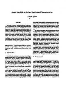
3. Problem formulation Siebesma and Holtslag (1996) already demonstrated that a well-chosen constant detrainment and entrainment rate can adequately reproduce the observed steady-state profiles such as observed during BOMEX. Indeed, the standard parameterization described in the previous section with fixed mixing rates (i.e., ␧ ⫽ ce z⫺1 m⫺1 with ce ⫽ 1.0 and ␦ ⫽ 2.75 ⫻ 10⫺3 m⫺1) produces almost perfect steady-state ␪ and qt profiles close to the observations (not shown). This result is not surprising since the choices of the entrainment and the detrainment rates are directly inspired by the diagnosed mixing rates as obtained from LES results based on BOMEX (Siebesma et al. 2003). The central and more interesting issue that we want to address in this paper is to what extent a simple parameterization with fixed entrainment and detrainment rates can be applied to more complicated cases such as the ARM diurnal cycle. In Fig. 1 we show for the ARM case time series of total water specific humidity qt in the subcloud layer at 300 m and at two heights in the cloud layer (1300 and 2100 m) for both the LES and the SCM results with the standard parameterization. The simple observation that can be made from these time series is that, in the latter half of the cloudy period (from 1000 to 1930 LT), the

FEBRUARY 2008

563

DE ROOY AND SIEBESMA

FIG. 2. Total water specific humidity profiles for different simulation hours during the ARM case for the LES model and the standard SCM using the default fixed ␧ and ␦.

plume model (Betts 1975), which reads for moist conserved variables: FIG. 1. Time series of total water specific humidity during the ARM case at three levels (300, 1300, and 2100 m) for LES and for the standard SCM using the default fixed ␧ and ␦.

SCM overestimates the humidity in the subcloud layer and in the lower half of the cloud layer while the humidity in the upper half of the cloud layer is underestimated. This suggests that for this case, the parameterized convective transport in the SCM is not active enough. This is also demonstrated in Fig. 2, in which the humidity profile is shown for both the LES and SCM results at 1930 LT (0030 UTC). Similar results (not shown) are obtained for the potential liquid water temperature ␪ᐉ . The aforementioned discrepancies between SCM and the LES results for the ARM case are also present in the SCM results reported in Soares et al. (2004), who used ␧ ⫽ 2 ⫻ 10⫺3 and ␦ ⫽ 3 ⫻ 10⫺3 m⫺1. To explain and understand these differences between the LES data and SCM results, we need to take a closer look at the lateral exchange rates such as those diagnosed in the LES model. This will be the topic of the next section.

4. Lateral mixing as diagnosed by LES To diagnose bulk lateral entrainment and detrainment from LES results one can use a simple entraining

⭸␾u ⫽ ⫺␧共␾u ⫺ ␾兲, ⭸z

共3兲

where ␾ refers to either the liquid water potential temperature ␪ᐉ or the total water specific humidity qt. The cloudy updraft variables ␾u (where u stands for updraft) and the mass flux can be easily diagnosed through conditional sampling of the LES output. Subsequently, the fractional entrainment and detrainment rates can be determined through the use of (3) and (1). Throughout this study we only use the so-called cloudcore sampling, in which the cloudy updraft is defined as all the LES grid points that contain liquid water (ql ⬎ 0) and are positively buoyant (␪␷ ⬎ ␪␷). Here ␪␷ is the virtual potential temperature and ␪ ␷ is the slabaveraged virtual potential temperature. The cloud-core sampling method is chosen because it describes the turbulent fluxes the best (SC95). It should be understood that for the remainder of this study “cloud core” will be referred to as “updraft.” For the analysis of the LES results in this section we will use the hourly averaged output of the ARM case, as this case contains a wide variety of cloud depths and environmental conditions. Figure 3 displays the LES diagnosed fractional entrainment and detrainment rates. It appears that the variation in ␦ during the simulation is much larger than for ␧ (note the different x-axis scale). The limited variation in ␧ might be related to the presence of a protecting shell around the cloudy core (Zhao and Austin

564

MONTHLY WEATHER REVIEW

VOLUME 136

FIG. 3. Hourly averaged fractional (a) entrainment and (b) detrainment rates diagnosed from LES results for the ARM case. Note the different x-axis scales for (a) and (b).

2005a,b) with properties in between core and environmental values. Because of this shell the influence of the environment on the cloudy core is damped, leading to a relative insensitivity of ␧ for the environment. A more quantitative way to look at the (in) sensitivity of ␧ and ␦ is to compare the directly diagnosed mass fluxes from the LES with (i) the mass flux obtained using a fixed parameterized fractional entrainment rate ␧ ⫽ ce z⫺1 along with the dynamical LES diagnosed fractional detrainment rate ␦ (Fig. 4a) and (ii) the mass flux obtained using a fixed parameterized fractional de-

trainment rate ␦ ⫽ 2.75 ⫻ 10⫺3 along with the dynamical LES diagnosed fractional entrainment rate (Fig. 4b). This clearly shows that the fixed parameterized fractional entrainment profile along with hourly diagnosed fractional detrainment rates gives an excellent estimate of the mass fluxes. Conversely the combination of a dynamical LES diagnosed entrainment rate with the fixed fractional detrainment rate results in considerable scatter, with under- and overestimations of the mass flux. So, it seems more useful to concentrate on improving the mass flux profile by developing a

FIG. 4. Comparison of the mass flux for the ARM case as directly diagnosed from LES with (a) the mass flux obtained using a fixed parameterized fractional entrainment rate (␧ ⫽ z⫺1) along with the dynamical LESdiagnosed ␦, or (b) with the mass flux obtained using a fixed parameterized fractional detrainment rate (␦ ⫽ 2.75 ⫻ 10⫺3) along with the dynamical LES-diagnosed ␧.

FEBRUARY 2008

DE ROOY AND SIEBESMA

FIG. 5. Mean detrainment rates (averaged over the cloud layer) diagnosed from LES results for the ARM case.

more dynamical ␦ parameterization. Therefore, we will use a fixed function for ␧ and develop a dynamical detrainment formulation to produce the correct mass flux profiles. The above-mentioned results are consistent

565

with Jonker et al. (2006) who showed that, for an LES study based on the small cumulus microphysics study (SCMS) experiment (Neggers et al. 2003), the variation with cloud size of ␧ is an order of magnitude smaller than for ␦. Figure 5 presents the cloud-layer-height dependence of the LES fractional detrainment rate averaged over the cloud layer (noted as 具␦LES典). Most striking is the decrease of ␦ with increasing cloud height until 1530 LT. This can be explained as follows (see Fig. 6). Many studies considering shallow convection (e.g., SC95) showed that ␦ is larger than ␧. Consequently, the mass flux profile decreases with height, reflecting an ensemble of clouds with more shallow clouds losing their mass at relatively low heights, and larger clouds transporting mass in the upper part of the cloud layer (SC95). Constant entrainment and detrainment rates (e.g., the ones in our SCM) fix the mass loss per meter. In fact, it is the difference between ␧ and ␦ [see (1)] that determines how fast the mass flux decreases with height, and the diagnosed values from SC95 are such that the mass flux profile decreases monotonically to zero for a cloud depth of 1000 m (i.e., the cloud depth observed during BOMEX). However, a bold applica-

FIG. 6. Cloud ensembles for different cloud-layer depths and the corresponding mass flux profiles using fixed ␧ and ␦ based on a cloud-layer depth of 1000 m.

566

MONTHLY WEATHER REVIEW

tion of these rates on a shallower cloud layer will result in a nonzero mass flux at the cloud top, while applying these rates on a deeper cloud layer will result in a zero mass flux below cloud top (see Fig. 6), all in disagreement with LES model results. The remedy to this unwanted behavior is also clear: the difference between the entrainment and the detrainment needs to be chosen such that the resulting mass flux is exhausted around the cloud top, a suggestion already made in Siebesma (1998). With a fixed ␧, this calls for smaller detrainment rates for deeper cloud layers and larger detrainment rates for shallower clouds, all in qualitative agreement with the diagnosed detrainment rates displayed in Fig. 5. A second interesting feature that can be observed in Fig. 5 is that after simulation hour 9 (1530 LT), the cloud height decreases without an increase in detrainment. A plausible explanation of this phenomenon is that for these hours, the clouds rise in an environment that has already been premoistened for several hours by detrainment from former clouds (see also Raymond and Blyth 1986). Therefore the entrained air will be moister, and hence less evaporative cooling will occur, resulting in lower detrainment rates than in a drier environment. This effect has been demonstrated recently in great detail by Derbyshire et al. (2004), where they studied convective activity in a number of cases in which only the environmental relative humidity was varied. A good measure of this effect can be expressed by the critical fraction of environmental air ␹c (Kain and Fritsch 1990), a parameter coming from the buoyancy-sorting concept. So, besides the detrainment rates, Fig. 5 also shows the analytically determined (see appendix A) mean critical fractions 具 ␹c 典 (averaged over the cloud layer). Let us first elucidate the meaning of ␹c with Fig. 7. Plotted is the virtual potential temperature ␪␷ of a mixture of updraft air with a fraction ␹ of environmental air. For pure updraft air, ␹ ⫽ 0 and obviously ␪␷(␹ ⫽ 0) ⫽ ␪␷,u. Likewise for ␹ ⫽ 1, the mixture consists of purely environmental air and ␪␷(␹ ⫽ 1) ⫽ ␪␷,e (where the subscript e stands for environment). Because of the evaporative cooling due to the mixing process, the mixing line is not just a straight line from ␪␷,u to ␪␷,e, but instead typically exhibits a minimum at the point where all the liquid water is evaporated. The critical fraction ␹c is defined as the fraction of environmental air that is needed to make the mixture neutrally buoyant. The heart of the Kain–Fritsch scheme is its assumption that all negatively buoyant mixtures (i.e., mixtures with ␹ ⬎ ␹c) will be detrained, while all positively buoyant mixtures (i.e., ␹ ⬍ ␹c) are entrained into the cloudy updraft. Consequently, if the environmental air is drier and/or

VOLUME 136

FIG. 7. The virtual potential temperature of a mixture of updraft air with environmental air as a function of the fraction ␹ of environmental air. The virtual potential temperature of the updraft and environmental air is ␪␷u and ␪␷e, respectively. Here ␹c is the fraction of environmental air necessary to make the updraft air just neutrally buoyant.

the buoyancy excess (␪␷,u ⫺ ␪␷,e) is smaller, ␹c will be smaller and hence the fractional detrainment rate will be larger. Here we see that also an updraft property itself (viz., ␪␷,u) is involved in what we will still call the dependence on environmental conditions. To recapitulate, the mean fractional detrainment rates shown in Fig. 5 are influenced by cloud height and environmental conditions. The two variables that can take this dependence into account are cloud depth h ⫽ zt ⫺ zb, where zt indicates cloud-top height, and the critical fraction ␹c. To investigate these dependencies on the mass flux profiles separately, Fig. 8a shows the nondimensionalized mass flux m ˆ ⫽ M/Mb as a function of the nondimensionalized height zˆ ⫽ (z ⫺ zb)/h, where zb is defined as the height with maximum mass flux. By rescaling the height by the cloud depth, we filtered out the effect of cloud depth on the detrainment. If cloud depth were the only parameter that determined ␦, Fig. 8a would display a data collapse. Instead we still observe a variation in the shape of the mass flux profile that is likely due to the different environmental conditions measured by 具 ␹c 典. Indeed, as expected we observe that larger values of 具 ␹c 典 lead to a relatively slower decrease of the mass flux profile and vice versa. This observation is in clear conflict with the standard parameterization (i.e., ␧ ⫽ z⫺1 and ␦ ⫽ 2.75 ⫻ 10⫺3 m⫺1). This is illustrated in Fig. 8b, in which the hourly averaged nondimensionalized mass fluxes are calculated using the ARM LES results for Mb, zb, and zt, but otherwise are constructed using the fractional entrainment and detrainment rates as given by the standard parameterization. This parameterization leads to erroneous mass flux profiles as can be clearly observed

FEBRUARY 2008

567

DE ROOY AND SIEBESMA

FIG. 8. (a) LES nondimensionalized mass flux profiles for the ARM case for different simulation hours (symbols as in Fig. 3). Here zb is defined as the height with maximum mass flux. (b) As in (a), but diagnosed with Mb, zb, and zt from the LES model in combination with ␧ ⫽ z⫺1 and ␦ ⫽ 2.75 ⫻ 10⫺3 m⫺1.

when comparing the parameterized mass flux profiles in Fig. 8b with the LES-derived mass flux profiles such as those displayed in Fig. 8a. In fact these discrepancies explain, consistent with Fig. 6, that for relatively shallow clouds the mass flux does not decrease rapidly enough, whereas it decreases too rapidly for the deepest clouds. The latter also finally explains the tooinactive convection in the SCM during the second half of the cloudy period of ARM, as discussed for Figs. 1 and 2.

a. Setup of the new parameterization In the previous section it has been shown that the mass flux profile is dependent on cloud-layer depth as well as on the environmental conditions measured by the ␹c parameter. Since the fractional entrainment does not vary nearly as much as the fractional detrainment rates from case to case, we keep the fractional entrainment formulation as in the standard parameterization (i.e., ␧ ⫽ ce z⫺1 with ce ⫽ 1.0), in reasonable agreement with LES results (also for other cases such as BOMEX and RICO). In order to have a more flexible mass flux formulation, we have to construct a simple parameterization for the fractional detrainment rate ␦. The simplest parameterization for ␦ to guarantee a zero mass flux at the cloud top is (Siebesma 1998) 1 , zt ⫺ z

冉

冊

1 1 dM ⫽ ce ⫺ ␦ dz, M z

5. A new detrainment parameterization

␦ ⫽ ␧共z兲 ⫹

which results in a linear decrease of the mass flux that can be checked easily by substituting (4) into (1). This parameterization already takes into account the cloudlayer-height dependence, but is still insensitive to the dependencies of the mass flux on the environment such as displayed in Fig. 8a. To include this effect we start with another approach. Let us assume for the time being that ␦ is constant with height (roughly following the LES results) and rewrite the mass continuity equation in (1) as

共4兲

共5兲

where we have substituted ␧ ⫽ ce z⫺1. This differential equation can be solved easily, using M(zb) ⫽ Mb as a lower boundary condition leading to M ⫽ Mb

冉冊 z zb

ce

e⫺␦共z⫺zb兲.

共6兲

Alternatively, we can nondimensionalize this form through zˆ and m ˆ (defined in section 4) so that

冋冉 冊 册

m ˆ ⫽ zˆ

h ⫹1 zb

ce

e⫺␦hzˆ ,

共7兲

or, if we invert it, we find for the fractional detrainment rate:

冉

冊

h ⫺ lnm ˆ ce ln 1 ⫹ zˆ zb ␦⫽ . hzˆ

共8兲

If we could come up with a parameterization of m ˆ at one specific height, we could plug this m ˆ into (8) to

568

MONTHLY WEATHER REVIEW

VOLUME 136

FIG. 10. LES results showing the relation between m ˆ and 具 ␹c 典 * * for RICO, BOMEX, and ARM. The dotted line represents a linear approximation of this relation [(9)]. FIG. 9. Nondimensionalized mass flux profiles for different simulation hours (ARM case) as in Fig. 8a but with ␧ ⫽ z⫺1 m⫺1 and ␦ according to (8) with Mb, zb, zt, and m ˆ as diagnosed from * LES. Above zˆ , a linearly decreasing mass flux profile is pre* scribed (see text).

obtain the optimal value of a constant fractional detrainment rate ␦. Preferably we should choose m ˆ at a height at which the differences between the various mass fluxes, such as those displayed in Fig. 8a, are most pronounced. Figure 8a suggests choosing m ˆ in the middle of the cloud layer (i.e., at zˆ ⫽ 0.5), and we will do so accordingly. Hereinafter the nondimensionalized height and mass flux in the middle of the cloud layer are denoted as zˆ and m ˆ , respectively. * * To show the potential of this approach, Fig. 9 displays the parameterized nondimensionalized mass flux profiles using for zˆ ⬍ 0.5 a constant fractional detrainment rate obtained by (8) with m ˆ , Mb , zb , and zt , all * diagnosed by the LES model. Comparing Fig. 9 with Fig. 8a shows that an optimal choice of a constant ␦ in the lower half of the cloud layer results in a realistic transition from a convex mass flux profile for small values of m ˆ to a concave profile for large m ˆ . To en* * sure that the mass flux goes smoothly to zero between zˆ ⫽ 0.5 and zˆ ⫽ 1, we simply impose a linear decrease of the mass flux profile to zero at the cloud top by applying (4) in the upper half of the cloud layer. At first sight, this last step might seem to be a crude approximation. However, Fig. 8a reveals that for small m ˆ * there is not much mass flux to spread out anymore, and for large m ˆ the linear decrease seems to be a reason* able approach [in agreement with, e.g., Jonker et al. (2006), Derbyshire et al. (2004), and Zhao and Austin (2005a)]. Although we believe that the first-order improve-

ments are well included with the proposed setup of the parameterization, there is certainly room for improvement of the parameterization in the upper half of the cloud layer. For example, it is plausible that the decrease of the nondimensionalized mass flux in the upper half of the cloud layer depends on ␹c. Another disadvantage of the current setup might be the incapability to produce a constant mass flux profile with height in the upper half of the cloud layer. However, in practice we expect this to be a rare, if not nonexistent, circumstance for shallow convection. The main question that remains is how to determine m ˆ and thereby close our parameterization. The sim* plest approach is to apply a well-chosen constant m ˆ * (e.g., 0.3; see Fig. 8a). Now the nondimensionalized mass flux profile is fixed and insensitive to dependencies of the mass flux on the environment. However, this already results in a large improvement in comparison with the standard parameterization with a fixed ␦ (see Fig. 8b), whereas the parameterization is equally simple. This improvement is caused by the cloud-layerheight dependence included in (8). Nevertheless the LES results of the former section clearly suggest parameterizing m ˆ as a function of ␹c. If we consider * clouds as updrafts, it is plausible that the mass flux decrease with height is influenced by ␹c on the way. Since we want to parameterize the fraction of the mass flux that is left in the middle of the cloud layer m ˆ , we * therefore average ␹c from the cloud base up to zˆ , and * we will denote this average for the remainder of this paper as 具 ␹c 典 . Instead of showing the nondimension* alized mass flux profiles together with 具 ␹c 典 for all * cases, the results are compendiously presented in Fig. 10 showing the dependence of m ˆ on 具 ␹c 典 according to * *

FEBRUARY 2008

DE ROOY AND SIEBESMA

the LES results for BOMEX, ARM, and RICO. Figure 10 reveals a clear correlation between 具 ␹c 典 and m ˆ * * with, as could be expected, a rapid decrease of the mass flux profile (i.e., small m ˆ ) for low values of 具 ␹c 典 , and * * vice versa. In practice, large values of 具 ␹c 典 can be as* sociated with large clouds (of large radii) with high updraft velocities that have large buoyancy excesses and/ or clouds rising in a friendly, humid environment. For small 具 ␹c 典 values the opposite can be expected. This * physical picture is consistent with results from the literature (see, e.g., Jonker et al. 2006; Zhao and Austin 2005a), which reveal a clear increase of m ˆ with increas* ing cloud sizes. It is also interesting to examine the potential of the relative humidity of the environment as an alternative indicator to describe the mass flux decrease with height. Figure 11 demonstrates the absence of any significant correlation between relative humidity and m ˆ . This can * be understood as follows. Normally relative humidity decreases with height, and consequently, low shallow clouds can go together with high values of averaged relative humidity. However, from our LES results we know that these types of clouds, present shortly after the beginning of convection in the ARM case, can show a rapid decrease of the mass flux, probably due to their small buoyancy excess. Here we see that high values of mean relative humidity can go together with a rapid decrease of the mass flux. This again demonstrates the necessity for including the effect of not only environmental humidity, but also buoyancy excess (as in 具 ␹c 典 ) * to adequately parameterize variations in the nondimensionalized mass flux profile. The last step is to find a parameterization for m ˆ * depending on 具 ␹c 典 in order to close our scheme. The * question is, to what extent is the LES relation between 具 ␹c 典 and m ˆ presented in Fig. 10 also applicable in an * * SCM? Although the ␹c profiles in our SCM, including the relative changes from hour to hour and case to case, resemble the LES profiles and changes, there are also differences. These differences are related to the explicit (cloud core) updraft definition in the LES model and the implicit updraft definition in an SCM. For instance, in the LES model, the updrafts start at the level of free convection (LFC) determined by the level where the updrafts become just neutrally buoyant and thus have zero ␹c values. From this height, the mass flux increases to a maximum at a level that is defined as the cloudbase height in this paper. In the SCM on the other hand, the mass flux starts and is at its maximum at the lifting condensation level (LCL). At this height the excess of the updraft properties, which influences the value of ␹c, is determined by the convection triggering parameterization. Consequently, ␹c already has a posi-

569

FIG. 11. As in Fig. 10, but now with the relative humidity averaged over the lower half of the cloud layer instead of 具 ␹c 典 . *

tive value at the cloud base (LCL in the SCM). This difference in updraft excess at the cloud base between SCM and LES model also affects higher levels. In practice, this leads to somewhat higher 具 ␹c 典 values in the * SCM compared to the LES model, mainly depending on the chosen convection triggering parameterization. Two approaches can be followed to deal with the above mentioned discrepancy. First, simply apply the LES relation between 具 ␹c 典 and m ˆ (Fig. 10) unaltered in the * * SCM. Second—this approach will probably be favored in an operational environment—adapt the relation between 具 ␹c 典 and m ˆ to the SCM (e.g., with a tuning * * based on one or more suitable 1D shallow convection cases). For soundness we follow the first approach. Consequently, as the 具 ␹c 典 values are higher in the * SCM, this will lead to a somewhat overactive convection scheme. Nevertheless, as we will see, the results are still good with large improvements in comparison with the standard parameterization. To make the cloud-base definitions in the LES and the SCM more comparable we start the averaging of ␹c in the SCM one model level above the LCL. The LES relation between 具 ␹c 典 and m ˆ is approximated by a * * linear fit for 具 ␹c 典 values larger than 0.2 and a small * minimum value of 0.05, resulting in the following expression for the SCM (see also Fig. 10): m ˆ ⫽ max共0.05, 5.24具␹c典 ⫺ 0.89兲. * *

共9兲

This result, combined with (8), finally completes our proposed detrainment parameterization. An interesting and positive characteristic of the new detrainment parameterization is the stabilizing effect through negative feedbacks. This is illustrated in Fig. 12. If an initial profile of temperature or humidity is

570

MONTHLY WEATHER REVIEW

FIG. 12. Schematic showing the stabilizing effect (negative feedback) of the new detrainment parameterization on perturbations in the humidity. The solid line represents the initial humidity profile while the dotted and dashed lines show the perturbed drier and moister profiles, respectively. The arrows indicate the shifting of the perturbed profiles owing to the changed, ␹c-dependent detrainment rates. Similar arguments apply for temperature instead of humidity. See the text for a more detailed explanation.

changed, the parameterization tries to compensate for the disturbance. If, for example, a humidity profile becomes drier, ␹c will decrease, leading to a larger fractional detrainment and consequently an increased moistening of the environment (see Fig. 12). Similar arguments apply for temperature. As a result, the parameterization works towards an equilibrium state. Finally, Fig. 13 shows how the new parameterization is embedded in the convection scheme. Note that the convection scheme is purely sequential, without any multiple iterations.

b. SCM results with the new detrainment parameterization Applying the new detrainment parameterization (8) in combination with (9) for zˆ ⬍ zˆ and (4) for zˆ ⬎ zˆ in * * our SCM, we run the BOMEX, ARM, and RICO cases. As mentioned in section 3, the standard parameterization as derived from LES for BOMEX leads to almost perfect steady-state humidity and temperature profiles for BOMEX. With the new detrainment parameterization, the humidity and temperature profiles are highly comparable for this case (not shown). As explained before, the ARM case poses stronger demands on the detrainment parameterization because the cloud height and the environmental conditions vary substantially during this case. Figures 14 and 15 with the new detrainment formulation reveal the clear improvements in the time series and profile of the total water

VOLUME 136

specific humidity in comparison with the corresponding Figs. 1 and 2 using the standard parameterization. Stronger convection during the second half of the cloudy period results in less humidity near the cloud base and more humidity in the upper part of the cloud layer, in accordance with the LES. However, there is no clear improvement with the new parameterization in the subcloud layer. This problem is probably not related to the lateral mixing in the cloud layer. One remark needs to be made in relation to Fig. 15. Since in the ARM case both the LES and the SCM are subjected to the same prescribed moisture surface fluxes, the vertical integrated moisture profile should be the same for both models. That this is not the case can be observed in Fig. 15 and is due to the fact that the LES models are usually formulated within the Boussinesq approximation, which assumes a constant horizontally averaged density, whereas in the SCM the decrease of density with height is taken into account. As is shown in appendix B, this causes small discrepancies between the moisture budgets of both models that deteriorate with time. However, it suffices here to note that these discrepancies do not affect any of the conclusions drawn in this study. Finally, Fig. 16 presents the results of the RICO case with LES, the standard and the new detrainment parameterization, and an imposed linear decreasing mass flux profile [i.e., (4) throughout the cloud layer]. We only show the profile after 24 h of simulation because other simulation hours just give “in-between results.” The new parameterization gives a very good match with the LES humidity profile although as expected, the convective activity is somewhat overestimated because the relation (9) derived from LES results is not optimized for our SCM, leading to a slight underestimation of the humidity at the cloud base. There is also a large improvement in the results in comparison with the standard parameterization. This can be explained by the relatively deep and moist cloud layer in the RICO case, leading to a slow decrease of the mass flux profile (see Fig. 10) and significantly smaller fractional detrainment values as for the BOMEX case. Finally, the results with the imposed linearly decreasing mass flux profile show that the included cloud height dependence results in increased convective activity and consequently better results in comparison with the standard parameterization. However, the convective activity is still underestimated as this parameterization does not deal with the favorable conditions for updrafts during the RICO case (high 具 ␹c 典 values). This illustrates the additional value * of the 具 ␹c 典 dependence in the new detrainment pa* rameterization.

FEBRUARY 2008

DE ROOY AND SIEBESMA

571

FIG. 13. Flowchart showing how the new parameterization is embedded in the convection scheme: ␾ ⫽ {␪l, qt}.

6. Discussion and conclusions A correct simulation of the mass flux profile is very important because it determines the vertical transport of the thermodynamic variables. Apart from the mass flux closure at the cloud base, the mass flux profile is determined by both the fractional entrainment and detrainment coefficients. LES results show that, for different cases and conditions, the fractional entrainment coefficient shows little variation. On the other hand, LES results also reveal much more variation in the detrainment coefficient; its value seems to depend mainly on two factors. First, and probably most important, is the dependence on the cloud-layer depth. Under normal conditions a shallow convection scheme in an NWP or climate model represents an ensemble of clouds, leading to a decreasing mass flux profile with height and zero mass flux at the top of the cloud layer (SC95). With an approximately fixed function for the entrainment coef-

ficient, it can be simply understood that this calls for smaller detrainment rates for deeper cloud layers, as also confirmed by LES. Nevertheless, current mass flux schemes ignore this cloud height dependence. We have shown that this can lead to large discrepancies with LES mass flux profiles. In our approach, the mass flux profile is considered in a nondimensionalized way, thereby dealing with the effect of the cloud-layer height. Already in its simplest form (i.e., a fixed function for ␧ and the new ␦ formulation with only one constant parameter) our approach deals with the cloudlayer-depth dependence, leading to a substantial improvement in comparison with fixed ␧ and ␦. The second important factor that influences ␦ is the environmental condition. Many studies (e.g., Kain and Fritsch 1990; Derbyshire et al. 2004) showed the influence of the relative humidity of the environmental air surrounding the updrafts. If the surrounding air is moister, less evaporative cooling will occur if this air is mixed with cloudy air, and this leads to less detrain-

572

MONTHLY WEATHER REVIEW

VOLUME 136

FIG. 15. Total water specific humidity profiles for different simulation hours during the ARM case for the LES model and the SCM with the new detrainment parameterization.

FIG. 14. Time series of total water specific humidity during the ARM case at three levels (300, 1300, and 2100 m) for LES and for the SCM using the new detrainment parameterization.

ment. However, besides the humidity of the environment, the buoyancy excess of the updraft air also determines if the mixture becomes negatively buoyant and consequently detrains. This combined effect is nicely captured by the so-called critical fraction of the environmental air, ␹c (Kain and Fritsch 1990). Indeed LES shows that the nondimensionalized mass flux profile, which is insensitive for cloud-layer height, correlates well with the ␹c profile. With the dependence of ␦ on ␹c we implicitly also include the effect that clouds with a larger radius or a higher updraft velocity will detrain less because larger clouds or clouds with a higher updraft velocity will normally also have a larger buoyancy excess and consequently higher ␹c values. Since Kain and Fritsch (1990) introduced their convection scheme based on the buoyancy-sorting concept, different modifications have been proposed in the literature and have been applied in operational NWP models (see, e.g., Bretherton et al. 2004; Kain 2004). Yet some important deficiencies with these types of schemes remain. In a Kain–Fritsch-like buoyancysorting scheme, mixtures are made of in-cloud and environmental air. Subsequently, all negatively buoyant mixtures detrain and positively buoyant mixtures en-

train. The amount of entrained and detrained air is strongly influenced by the fraction of the mass flux that is used for mixing [the rate of environmental inflow (REI)] and the probability density function (PDF), which describes the probability of different mixtures. Both influences are extreme simplifications of the mixing process in nature, which is, as we know from Zhao and Austin (2005a,b), quite complex. For example, the

FIG. 16. Total water specific humidity profiles after 24 h of simulation during the RICO case for the LES model and the SCM using fixed ␧ and ␦, the new detrainment parameterization, and an imposed linear decreasing mass flux profile [i.e., (4) throughout the cloud layer].

FEBRUARY 2008

573

DE ROOY AND SIEBESMA

entrained air does not have purely environmental but rather in-between properties. Apart from the abovementioned considerations, we should also realize that for common horizontal model resolutions a convection scheme describes an ensemble of clouds instead of one single updraft. All in all, it seems unlikely that parameters and functions like the PDF of the mixtures can be related to observations or LES results. Instead they can be seen as ways to tune the convection scheme. In our approach we take a step back in complexity (strongly reducing the tunable parameters) and relate the nondimensionalized mass flux profile directly to just one parameter, a bulk ␹c that, for several substantiated reasons, shows a clear correlation with the decrease of the nondimensionalized mass flux profile. Note that by fixing the function of the entrainment coefficient, we also circumvent the problem in current buoyancy-sortingbased lateral mixing schemes that a drier environment leads to less entrainment and consequently higher cloud tops; this is in disagreement with LES. A critical reader might wonder to what extent the cloud-base mass flux parameterization in (2) influences the results in this paper. To answer this we reproduced all SCM results but now applied the Grant (2001) cloud-base mass flux closure (see section 2a). The result is that all conclusions in this paper remain in full force. With the new detrainment parameterization included in an SCM, good results are obtained for all three investigated shallow convection cases. The complex ARM case, with increasing cloud height and changing environmental conditions, clearly reveals the shortcomings of fixed ␧ and ␦ and the substantial improvement with the new parameterization. For the steady-state BOMEX case, for which the fixed ␧ and ␦ are more or less optimized, the results with the new parameterization are equally good. Finally, the RICO case with a relatively deep and moist cloud layer demands small fractional detrainment rates. Hence, the new parameterization, which results in a very good match with LES, substantially improves the vertical mixing due to convection in comparison with the standard mixing model. By coupling the nondimensionalized mass flux profile directly to a bulk ␹c, the proposed detrainment parameterization can be seen as an alternative for more complex existing buoyancy-sorting-based convection schemes, without showing some of the disadvantages. Results from LES and an SCM show the clear potential of our approach for a wide range of shallow convection cases. Moreover, the proposed parameterization is computationally cheap and can be easily included in an existing mass flux scheme.

Acknowledgments. The authors thank Geert Lenderink, Stephan de Roode, Kees Kok, and Jan Fokke Meirink for stimulating and useful discussions. Geert Lenderink, Stephan de Roode, one anonymous referee, and Jack Kain are acknowledged for critical reading of, and useful suggestions for, an earlier version of this paper. Margreet van Zanten is thanked for providing the LES results for RICO.

APPENDIX A An Analytical Expression for ␹c The calculation of the critical fraction ␹c can, of course, be done numerically. Here we present, as an alternative, the derivation of an analytical expression of ␹c solely in terms of environmental and updraft fields. Such an analytical result has the advantage of making the convection parameterization computationally more efficient. Another advantage of such an analytical expression is that it provides more insight into the way ␹c, and hence the detrainment, reacts to the environmental and updraft conditions. We start with the virtual potential temperature of a mixture consisting of a fraction ␹ of environmental air and a fraction of 1 ⫺ ␹ of updraft air:

␪␷共␹兲 ⫽ ␪共␹兲关1 ⫹ ␭q␷ 共␹兲 ⫺ ql 共␹兲兴,

共A1兲

where q␷ is the water vapor specific humidity and ␭ ⫽ R␷ /Rd ⫺ 1 ⬇ 0.61 with Rd and R␷ being the specific gas constants for dry and moist air, respectively. Further, we will use the total water specific humidity qt ⬅ q␷ ⫹ ql and the liquid water potential temperature ␪ᐉ , which reads in its linearized form

␪ᐉ ⬇ ␪ ⫺

Lql , cp␲

共A2兲

where L is the specific latent heat of vaporization, cp is the specific heat capacity of dry air at constant pressure, and ␲ ⬅ T/␪ is the Exner function. The advantage of the moist conserved variables ␪ᐉ and qt is that they mix linearly:

␪ᐉ 共␹兲 ⫽ ␪ᐉu ⫺ ␹共␪ᐉu ⫺ ␪ᐉe兲 ⬅ ␪ᐉu ⫺ ␹⌬␪ᐉ qt 共␹兲 ⫽ qtu ⫺ ␹共qtu ⫺ qte兲 ⬅ qtu ⫺ ␹⌬qt .

共A3兲

By eliminating q␷ and ␪ in (A1) in favor of the moist conserved variables and ignoring higher-order moisture terms, we readily find

␪␷共␹兲 ⫽ ␪ᐉ 共␹兲关1 ⫹ ␭qt 共␹兲 ⫺ 共1 ⫹ ␭兲ql 共␹兲兴 ⫹

L q 共␹兲. cp␲ ᐉ 共A4兲

574

MONTHLY WEATHER REVIEW

Since qᐉ is not a moist conserved variable, it does not obey a simple linear mixing line like (A3). Therefore, the last preparation that we need to make is to find an expression for ql(␹) in terms of updraft and environment variables. As long as the mixture contains liquid water we may write ql 共␹兲 ⫽ qt 共␹兲 ⫺ qs 关p, T共␹兲兴,

共A5兲

where qs is the saturation-specific humidity that depends on the temperature of the mixture and the pressure p. Because we want an expression for ␹c, it is enough to have an expression for ␪␷(␹) from ␹ ⫽ 0 to ␹ ⫽ ␹c, which ensures that ql ⬎ 0 and that (A5) is valid. We proceed by making a Taylor expansion of qs[T(␹)] around the T(␹ ⫽ 0) ⬅ Tu: qs 关T共␹兲兴 ⬇ qs 共Tu兲 ⫹ 关T共␹兲 ⫺ Tu 兴

⭸qs ⭸T

冏

.

共A6兲

Tu

By substituting (A6) back in (A5) and rewriting it in terms of moist conservative variables using (A2), we obtain 1 ql 共␹兲 ⫽ qlu ⫺ ␹ 共⌬qt ⫺ ␥⌬␪ᐉ兲, 1⫹␥

共A7兲

with ␥ ⫽ (L/cp)⳵qs/⳵T | Tu . We can now harvest by substituting (A7) and (A3) into (A4), and rewriting it as a linear combination of updraft excesses ⌬␪ᐉ and ⌬qt. By ignoring higher-order terms of ␹ and terms of the O(10⫺2) in the prefactor of ⌬␪ᐉ , we find after some algebra that

冋

册

L ␪␷共␹兲 ⫽ ␪␷u ⫺ ␹ ␤⌬␪ᐉ ⫹ 共␤ ⫺ ␣兲 ⌬q , cp␲ t

共A8兲

with

␤⬅

1 关1 ⫹ 共1 ⫹ ␭兲␥␣兴 and 1⫹␥

␣⬅

cp ␲␪ . L ᐉu

Typical values for the cases considered in this paper are ␥ ⯝ 2.5, ␣ ⯝ 0.12, and ␤ ⯝ 0.4. Realizing that ␹c is defined as the concentration of environmental air for which the buoyancy with respect to the environment is just zero, we finally find ⌬␪␷ ␹c ⫽ , 关␤⌬␪ᐉ ⫹ 共␤ ⫺ ␣兲L Ⲑ共cp␲兲⌬qt兴

共A9兲

where obviously ⌬␪␷ ⬅ (␪␷u ⫺ ␪␷e) denotes the updraft buoyancy excess. We have deliberately adopted the same notation as in Randall (1980) and Bretherton et al. (2004) except that we use ␣ and ␭ instead of ␧ and ␦

VOLUME 136

in order to avoid confusion with our notation for the fractional entrainment and detrainment rates. Note that in contrast with Bretherton et al. (2004) we find a slightly different form for the prefactor of the ⌬qt term and, more importantly, a different sign of this term. Comparison of (A9) with accurate numerical estimates of ␹c for typical values of the presented cases in this article shows that (A8) gives errors only of the order of 1%. To gain some more insight in the behavior of ␹c we can simplify the result in (A9) even more by assuming that Tu ⯝ T. This allows us to write the excess terms as ⌬␪ᐉ ⯝ ⫺

L q and cp␲ ᐉu

⌬qt ⯝ qte ⫺ qse ⫺ qᐉu.

共A10兲

Using these approximations of the excesses and the definition of the relative humidity RH ⬅ qte /qse allows us to rewrite (A9) as

␹c ⫽ 共cp␲ⲐL兲

⌬␪␷ qse共␤ ⫺ ␣兲共1 ⫺ RH兲 ⫺ ␣qᐉu

共A11兲

and to show how ␹c increases for larger buoyancy excess values and higher relative humidities.

APPENDIX B Differences in Tendencies between the LES Model and the SCM The DALES model used here is formulated, as are most LES models, within the Boussinesq approximation. This implies that the horizontally averaged density does not change with height. The SCM used in this study does take the height dependence of the density into account, as do all GCMs, RCMs, and their SCM versions. This difference has implications for the moisture tendencies and is hence a possible obstacle preventing precise comparisons between LES and SCM results. To quantify the difference, consider a tendency equation for moisture used in an SCM, containing a turbulent flux divergence term only:

冉 冊 ⭸q ⭸t

⫽⫺

1 ⭸␳ w⬘q⬘ ␳ ⭸z

⫽⫺

⭸w⬘q⬘ 1 ⭸␳ ⫺ w⬘q⬘ ⭸z ␳ ⭸z

SCM

⫽

冉 冊 ⭸q ⭸t

⫺ w⬘q⬘ LES

1 ⭸␳ . ␳ ⭸z

共B1兲

The last term on the right-hand side (the density term) quantifies the discrepancy in the moisture tendency if

FEBRUARY 2008

DE ROOY AND SIEBESMA

the height dependence of density is not taken into account. The term (1/ ␳)(⳵␳/⳵z) is of the order 10⫺4 m⫺1 in the lower troposphere. Furthermore, if we assume for the sake of simplicity that the moisture flux is linear, decreasing to zero between the surface and a dry boundary layer height zi, so that

冉 冊 ⭸q ⭸t

⯝ LES

共w⬘q⬘兲srf , zi

共B2兲

we can quantify the density term as w⬘q⬘

冉 冊

1 ⭸␳ ⭸q ⯝ 10⫺4共zi ⫺ z兲 ⭸t ␳ ⭸z

,

共B3兲

LES

which is as large as 10% at a height of only 1000 m with zi ⯝ 2000 m. If we realize that, for example, a moisture surface flux of 6 ⫻ 10⫺5 m s⫺1 moistens a boundary layer of 2000 m thick by 2.5 g kg⫺1 during a day, this implies that the density term is of the order of 0.25 g kg⫺1 over the entire depth; this value is comparable with the discrepancy that can be observed in Fig. 15. So we can conclude that if we compare LES results, which are based on the Boussinesq approximation, with SCM output, differences for the moisture budget may be expected which become significantly large beyond simulation periods of approximately 10 h. REFERENCES Betts, A. K., 1975: Parametric interpretation of trade-wind cumulus budget studies. J. Atmos. Sci., 32, 1934–1945. ——, and M. Miller, 1986: A new convective adjustment scheme. Part II: Single column tests using GATE wave, BOMEX and artic air-mass data sets. Quart. J. Roy. Meteor. Soc., 112, 677– 691. Bretherton, C. S., J. R. McCaa, and H. Grenier, 2004: A new parameterization for shallow cumulus convectionn and its application to marine subtropical cloud-topped boundary layers. Part I: Description and 1D results. Mon. Wea. Rev., 132, 864–882. Brown, A. R., and Coauthors, 2002: Large-eddy simulation of the diurnal cycle of shallow cumulus convection over land. Quart. J. Roy. Meteor. Soc., 128, 1075–1094. Cuijpers, J. W. M., and P. Bechtold, 1995: A simple parameterization of cloud water related variables for use in boundary layer models. J. Atmos. Sci., 52, 2486–2490. ——, and A. A. M. Holtslag, 1998: Impact of skewness and nonlocal effects on scalar and buoyancy fluxes in convective boundary layers. J. Atmos. Sci., 55, 151–162. Cuxart, J., P. Bougeault, and J.-L. Redelsperger, 2000: A turbulence scheme allowing for mesoscale and large-eddy simulations. Quart. J. Roy. Meteor. Soc., 126, 1–30. Derbyshire, S. H., I. Beau, P. Bechtold, J.-Y. Grandpeix, J.-M. Piriou, J.-L. Redelsperger, and P. M. M. Soares, 2004: Sensitivity of moist convection to environmental humidity. Quart. J. Roy. Meteor. Soc., 130, 3055–3079.

575

Grant, A. L. M., 2001: Cloud-base fluxes in the cumulus-capped boundary layer. Quart. J. Roy. Meteor. Soc., 127, 407–422. ——, and A. R. Brown, 1999: A simililarity hypothesis for shallow cumulus transports. Quart. J. Roy. Meteor. Soc., 125, 1913– 1936. Gregory, D., J.-J. Morcrette, C. Jakob, A. C. M. Beljaars, and T. Stockdale, 2000: Revision of convection, radiation and cloud schemes in the ECMWF Integrated Forecasting System. Quart. J. Roy. Meteor. Soc., 126, 1685–1710. Holland, J. Z., and E. M. Rasmusson, 1973: Measurement of atmospheric mass, energy and momentum budgets over a 500kilometer square of tropical ocean. Mon. Wea. Rev., 101, 44– 55. Jakob, C., 2003: An improved strategy for the evaluation of cloud parameterizations in GCMs. Bull. Amer. Meteor. Soc., 84, 1387–1401. ——, and A. P. Siebesma, 2003: A new subcloud model for massflux convection schemes: Influence on triggering, updraught properties, and model climate. Mon. Wea. Rev., 131, 2765– 2778. Janjic, Z. I., 1994: The step-mountain eta coordinate model: Further developments of the convection, viscous sublayer, and turbulence closure schemes. Mon. Wea. Rev., 122, 927–945. Jonker, H. J. J., R. A. Verzijlbergh, T. Heus, and A. P. Siebesma, 2006: The influence of the subcloud moisture field on cloud size distributions and the consequences for entrainment. Extended Abstracts, 17th Symp. on Boundary Layers and Turbulence, San Diego, CA, Amer. Meteor. Soc., 2.4. Jonker, S., 2005: Evaluation study of the Kain–Fritsch convection scheme. KNMI Tech. Rep. TR275, KNMI, 69 pp. Kain, J. S., 2004: The Kain–Fritsch convective parameterization: An update. J. Appl. Meteor., 43, 170–181. ——, and J. M. Fritsch, 1990: A one-dimensional entraining/ detraining plume model and its application in convective parameterization. J. Atmos. Sci., 47, 2784–2802. Lenderink, G., and A. P. Siebesma, 2000: Combining the massflux approach with a statistical cloud schemes. Preprints, 14th Symp. on Boundary Layers and Turbulence, Aspen, CO, Amer. Meteor. Soc., 66–69. ——, and A. A. M. Holtslag, 2004: An updated length-scale formulation for turbulent mixing in clear and cloudy boundary layers. Quart. J. Roy. Meteor. Soc., 130, 3405–3427. Neggers, R. A. J., A. P. Siebesma, and H. J. J. Jonker, 2002: A multiparcel method for shallow cumulus convection. J. Atmos. Sci., 59, 1655–1668. ——, P. G. Duynkerke, and S. M. A. Rodts, 2003: Shallow cumulus convection, a validation of large-eddy simulation against aircraft and Landsat observations. Quart. J. Roy. Meteor. Soc., 129, 2671–2696. ——, A. P. Siebesma, G. Lenderink, and A. A. M. Holtslag, 2004: An evaluation of mass flux closures for diurnal cycles of shallow cumulus. Mon. Wea. Rev., 132, 2525–2536. Randall, D. A., 1980: Conditional instability of the first kind upside-down. J. Atmos. Sci., 37, 125–130. ——, and Coauthors, 2003: Confronting models with data: The GEWEX Clouds Systems Study. Bull. Amer. Meteor. Soc., 84, 455–469. Raymond, D. J., and A. M. Blyth, 1986: A stochastic mixing model for nonprecipitating cumulus clouds. J. Atmos. Sci., 43, 2708–2718. Siebesma, A. P., 1998: Shallow cumulus convection. Buoyant Convection in Geophysical Flows, E. J. Plate et al., Eds., Vol. 513, Kluwer Academic, 441–486.

576

MONTHLY WEATHER REVIEW

——, and J. W. M. Cuijpers, 1995: Evaluation of parametric assumptions for shallow cumulus convection. J. Atmos. Sci., 52, 650–666. ——, and A. A. M. Holtslag, 1996: Model impacts of entrainment and detrainment rates in shallow cumulus convection. J. Atmos. Sci., 53, 2354–2364. ——, and Coauthors, 2003: A large eddy simulation intercomparison study of shallow cumulus convection. J. Atmos. Sci., 60, 1201–1219. Soares, P. M. M., P. M. A. Miranda, A. P. Siebesma, and J. Teixeira, 2004: An eddy-diffusivity/mass-flux parameterization for dry and shallow cumulus convection. Quart. J. Roy. Meteor. Soc., 130, 3365–3384.

VOLUME 136

Stevens, B., and Coauthors, 2001: Simulations of trade wind cumuli under a strong inversion. J. Atmos. Sci., 58, 1870–1891. Tiedtke, M., 1989: A comprehensive mass flux scheme for cumulus parameterization in large-scale models. Mon. Wea. Rev., 117, 1779–1800. Unden, P., and Coauthors, 2002: HIRLAM-5 scientific documentation. Tech. Rep., SMHI, 144 pp. Zhao, M., and P. H. Austin, 2005a: Life cycle of numerically simulated shallow cumulus clouds. Part I: Transport. J. Atmos. Sci., 62, 1269–1290. ——, and ——, 2005b: Life cycle of numerically simulated shallow cumulus clouds. Part II: Mixing dynamics. J. Atmos. Sci., 62, 1291–1310.