Department of Computer Science, University of Hertfordshire. College Lane, Hatfield ... or more history registers which store the outcome of k previous branches ...
A SIMPLE YET ACCURATE NEURAL BRANCH PREDICTOR S.P.Hunt, C.Egan, A.Shafarenko Department of Computer Science, University of Hertfordshire College Lane, Hatfield, Herts. AL10 9AB United Kingdom Email: {S.P.Hunt, C.Egan, A.Shafarenko}@herts.ac.uk
Abstract In this paper, we examine the application of simple neural processing elements to the problem of dynamic branch prediction in high-performance processors. A single neural network model is considered: the Perceptron. We demonstrate that a predictor based on the Perceptron can achieve a prediction accuracy in excess of that given by conventional Two-level Adaptive Predictors and suggest that neural predictors merit further investigation. Key Words Neural Networks, Computing, Engineering, Optimization
1
Introduction
Modern computer architectures employ techniques such as pipelining and multiple instruction issue to boost throughput. In principle, significant performance gains can be achieved by increasing pipeline depth and the number of instructions issued per clock cycle; however, in practice there are penalties for adopting such strategies. These penalties arise because real-world programs contain sequences of instructions that may give rise to structural hazards, control hazards or data hazards [1]; if these hazards are not taken into account in the design of a processor (and compilers that produce programs to run on it), many performance gains may be negated.
1.1 The Branch Prediction Problem Where a program contains a conditional branch instruction, it is necessary to know whether or not the condition is satisfied in order to determine which instruction should be fetched next; similarly, where a program contains a return statement or an indirect branch, it is necessary to determine the target address so that the next instruction can be fetched from the correct place. Both of these are examples of control hazards. The problem here is that the necessary information is not available early enough in the fetch-execute cycle to
ensure that the next instruction can be fetched in time to fill the next empty slot in the pipeline [1]. There are many approaches to this problem, the simplest of which is to wait until the information is available; however, this can drastically reduce throughput, especially in a processor that employs multiple instruction issue and deep pipelines. One of the most common alternatives to the wait-and-see approach is to attempt to predict whether or not a branch will be taken, and to predict the target address in the event that it is [1, 2]. One significant drawback of branch prediction is that an incorrect prediction will typically cause a longer delay than would have occurred had the processor simply waited for the condition to be evaluated. Thus, the level of accuracy achieved is very important [2].
1.2 Branch Predictors There are two broad classes of branch predictors: static branch predictors (in which the information used to make predictions does not change at run time) and dynamic branch predictors (in which the information is changed to reflect the fact that a program’s activity changes over time). Unsurprisingly, dynamic branch predictors give predictions that are more accurate than those provided by static branch predictors [3, 4]; however, they require more processing resources. Static branch predictors may make use of profile information, information from compile-time analysis, or information about branch direction or opcode [3]. A simple dynamic branch predictor would employ a two-bit saturating counter that is updated each time a conditional branch instruction is encountered: the most significant bit of the counter is used to furnish the prediction [2, 5]. However, more sophisticated branch predictors employ a two-level adaptive scheme: the first level comprises one or more history registers which store the outcome of k previous branches; the second level is a table of saturating counters which is indexed by a combination of the branch address and the contents of the history register [2, 5]. A branch predictor of this type learns to divide branch
instructions into two classes: “take” and “do not take”: this functionality is similar to that of a simple Perceptron or ADALINE [6].
2.1 Perceptron-Based Predictors
1.3 Neural Branch Predictors
One of the problems that is faced by the designer of a branch predictor is that the prediction should ideally be performed during the Instruction Fetch (IF) stage of the fetch-execute cycle. Unfortunately, at this point the only information we have about the instruction is its address, so we don’t even know whether or not a prediction should be performed. To circumvent this problem we employ a branch target cache, which is used to store information about previously-encountered branch instructions. The advantage of this is that the predictor should only be called upon when there is a conditional branch to resolve, and so its branch prediction performance will not be affected by attempts to learn how to predict the outcome of any other kind of instruction. The disadvantage is that it will not be able to make a prediction on the first occasion that a branch instruction is encountered.
Branch prediction is a pattern classification problem, whether the prediction is based upon static or dynamic data. Dynamic branch prediction is also an example of a time series prediction problem. Artificial neural networks are well known to be suited to solving problems in both such application areas [6, 7]; indeed, artificial neural networks have already been applied to the static branch prediction problem with some success [8, 9], and initial work on applying neural network techniques to dynamic branch prediction has shown some promising results [4, 10, 11]. If neural predictors are to be of practical use there are three questions that must be answered in the affirmative: • Can a neural network based branch predictor be constructed that is accurate enough to compete with a conventional branch predictor? • Can a hardware-based neural predictor be made to operate quickly enough for its predictions to be useful in a real CPU? • Can the hardware cost of a neural branch predictor be kept low enough for it to be a viable alternative to a conventional branch predictor? Whilst we are mindful of all of these questions, in this paper we seek to address only the first of them.
2
Experimental Models
We have chosen to investigate the branch prediction potential of one of the simplest of all neural network models: the Perceptron [6, 12]. We concentrate on this model precisely because it is so simple - in terms of both the operation of individual processing elements, and the application of the training algorithm that it employs. Generally, simplicity is a virtue where processor design is concerned: the more complex a functional unit is, the more difficult and costly it is likely be to realize it in hardware. Thus it makes sense to use the simplest type of neural network that we can.
2.1.1 How Predictions are Performed
At the heart of each predictor is a processing element (PE) with n numerical inputs (x1 .. xn), each of which has an associated weighting factor (w1 .. wn). The activation, a, of a PE is computed by summing its weighted inputs: n
a = ∑ wi xi i =0
where w0 is an additional weight known as the bias, and x0 is fixed at 1. The result is passed through a threshold function to calculate the output, y, of the PE:
⎪⎧high, if a ≥ 0⎪⎫ y= ⎨ ⎬ ⎪⎩low, if a < 0 ⎪⎭ where high is 1 and low is either 0 (for a binary PE) or -1 (for a bipolar PE). The resulting PE may be used as a classifier, with each input vector assigned to one of two classes, according to the output of the PE (high or low). In our branch predictor the two classes are interpreted as predict taken and predict not taken. Each of the input vectors that is passed to a predictor is an n-bit branch history, in which the values of the n bits represent whether the last n branches were taken or not taken. A branch history vector may be global (in which case it contains aggregate data about the last n branches), or it may be local (in which case it contains data about the last n occurrences of a single branch instruction), or it may be combined (in which case a global history and a local history are concatenated to create a single vector). These branch history data may be encoded in either a binary (0/1) or a bipolar (±1) form.
2.1.2 How Predictions Are Learned The classification of an input vector (and hence the prediction) depends on the PE’s weight vector, which is determined by training. Our predictors are trained by a technique known as the Perceptron Convergence Procedure (PCP), in which connection weights are initialized to 0, then input patterns are presented to the PE one at a time, and weight changes are made according to the following prescription:
⎧ ∆w = 0, if y is correct or x = 0⎫ i ⎪ i ⎪ ⎪ ⎪ ⎨ ∆wi = +α , if xi × t - y > 0 ⎬ ⎪ ⎪ ⎪⎩ ∆wi = −α , if xi × t - y < 0 ⎪⎭
( ) ( )
Here t is the target output (in this case either taken or not taken), and α is the learning rate associated with the PE. Thus, the weights on the connections into a predictor (its weight vector) will be changed every time it is found to have made a mis-prediction. Fortunately, the PCP is not particularly sensitive to leaning rate [6], so we are at liberty to choose a value for α on the basis that it is convenient from an implementation point of view. Given that our ultimate goal is to implement the neural predictor in hardware, the obvious choice for the learning rate is 1: by making this choice we guarantee that weight updates will be easy to perform in hardware, and we ensure that the weights will only take on integer values, so we can employ integer arithmetic throughout our predictor. It is worth noting two key features of the PCP at this point: the first is that a predictor’s weight vector will be changed if and only if it makes an incorrect prediction, and the second is that the size of a weight change does not depend on how much the system is in error. As a consequence of these features, PE’s trained via the PCP are quick to learn classification tasks and can be retrained almost as quickly. It is for this reason that the PCP (which was designed for off-line training with a static data set) is an appropriate learning algorithm for a dynamic problem such as branch prediction.
2.2 The Data The input to the simulator is a text file containing a program execution trace from which all of the non-branch instructions have been removed. Each line of the trace file contains three pieces of data: the value of the program counter, whether the branch was taken or not, and the target address for the branch, had it been taken. As this is a dynamic prediction task, the data from the trace file may
(and, indeed, should) be used both to train and to test the branch predictor. In order to test our predictors we extracted the conditional branches from a set of instruction traces for the Stanford integer benchmark suite. This is a collection of eight C programs designed to be representative of nonnumeric code. The benchmarks have an average dynamic instruction count of 273,000, about 18% of which are branches - of which around 76% are taken. Some of the branches in these benchmarks are known to be particularly difficult to predict; for example those in quicksort. [13] The benchmarks were compiled using a C compiler developed at the University of Hertfordshire for the HSA (Hatfield Superscalar Architecture) [14]. Instruction traces were generated using the HSA instruction-level simulator, and these were then modified for use with the neural predictor simulation software.
2.3 The Simulator We have constructed a simulator, using the Delphi 6 Integrated Development Environment. This simulator allows us to test the performance of predictors that employ global, local and combined branch histories of varying lengths. The simulator implements a single global predictor, a set of local predictors, or a set of combined (global + local) predictors. The global branch history length may be varied between 2 bits and 128 bits (in 2-bit increments), as may the branch history lengths for the set of local predictor. Combined predictors may be constructed with any combination of global and local history lengths. The simulator permits us to represent branch histories either in binary or in bipolar form. In each of the experiments reported here, we used a table of 1024 local predictors and a table of 1024 combined predictors. These tables are indexed by the program counter, so that each local or combined predictor is associated with a different set of branch instructions.
3
Results
The results of our experiments are summarized in figures 1 to 4. The graphs show the mean prediction accuracy for the predictors concerned when trained and tested on the full set of 8 programs from the Stanford integer benchmark suite. In each case this figure is an average of the prediction accuracy figures for the 8 benchmarks, weighted so as to take account of the different number of branches in each of the instruction traces.
3.1 Global Predictors 87%
Proportion Correct
Again, the best performance is achieved by predictors employing a 128 bit history, but this time there is a sufficient difference between the performance of binary and bipolar predictors (at 93.82% and 94.10% respectively) to be noticeable in practice.
3.3 Combined Predictors 97%
Proportion Correct
96%
95% Global History Length
94%
Global Predictor Performance
93%
86%
Local History Length
92% 8
Bipolar Data Binary Data
85%
Branch History Length
84% 8
16
24
32
40
48
56
64
72
80
88
16
24
32
40
48
56
64
72
80
88
8 16 24 32 64 96 128
96 104 112 120 128
Figure 3: Effect of branch history length on the prediction accuracy of bipolar perceptron-based predictors trained on combined global+local data. (1024 combined predictors, each trained with a combination of branch history data for a single branch and global history data)
96 104 112 120 128
Figure 1: Effect of branch history length on the prediction accuracy of perceptron-based predictors trained on global data. (Single predictor, aggregate branch history data)
The best performance here is achieved by global predictors employing a 128-bit history; furthermore, there is almost no difference between the performance of the predictors trained on binary and bipolar data, at 86.61% and 86.64% correct predictions respectively.
In this instance the best performance (96.41% correct) was achieved with a set of predictors, each of which combines 128 bits of global history with 108 bits of local history. 97%
Proportion Correct
96%
95%
3.2 Local Predictors 95%
Proportion Correct
Global History Length
94%
Local Predictor Performance
93% Local History Length
92% 94%
8
Bipolar Data Binary Data
93%
16
24
32
40
48
56
64
72
80
88
8 16 24 32 64 96 128
96 104 112 120 128
Figure 4: Effect of branch history length on the prediction accuracy of binary perceptron-based predictors trained on combined global+local data. (1024 combined predictors, each trained with a combination of branch history data for a single branch and global history data)
Branch History Length
92% 8
16
24
32
40
48
56
64
72
80
88
96 104 112 120 128
Figure 2: Effect of branch history length on the prediction accuracy of perceptron-based predictors trained on local data. (1024 local predictors, each trained with branch history data for a single branch instruction)
Here the best performance (95.72% correct) was achieved with a set of predictors, each of which combines 128 bits of global history with 78 bits of local history.
3.4 Results for Individual Benchmarks In almost all cases we find that the bipolar predictors perform better than binary predictors employing the same history lengths. For example, he prediction accuracy achieved for the different benchmarks varies quite widely (see Tables 1 and 2 below) Benchmark
Bubble Matrix Perm Puzzle Queens Sort Tower Tree Overall
Best accuracy 87.34% 99.80% 99.59% 97.66% 86.33% 74.41% 99.42% 89.56% 96.41%
Configuration Global History 122 10 68 128 128 22 80 42 128
Local History 124 30 100 76 128 2 112 34 108
Table 1: Highest prediction accuracy figures obtained for the 8 different benchmarks (combined predictors trained with bipolar data)
Benchmark
Bubble Matrix Perm Puzzle Queens Sort Tower Tree Overall
Best accuracy 86.24% 99.57% 99.42% 96.93% 84.97% 74.61% 99.27% 89.39% 95.72%
Configuration Global History 116 12 44 128 128 58 88 50 128
Local History 122 56 104 72 128 72 94 28 78
Table 2: Highest prediction accuracy figures obtained for the 8 different benchmarks (combined predictors trained with binary data)
As pointed out in Section 2.3, the outcomes of some branches are inherently more difficult to predict than others. For example, it is no surprise that we get what appears to be a very poor performance for Sort (an implementation of quicksort), since we know it to be amongst those algorithms that contains many difficult-topredict branches. [13]
4
Discussion
A number of points arise from this work. First, it is clearly possible to construct highly accurate neural branch
predictors using simple Perceptrons trained by the PCP. In previous work conducted in our Department [10], several different local and global two-level adaptive predictors were tested on the data set that has been used here. The most accurate global predictor was right approximately 90.5% of the time, whilst the best that could be managed by a local predictor was about 92.5%. On the face of it, the performance levels achieved by our Perceptron-based predictors are much higher than those available from more conventional predictors; however, it is worth sounding a note of caution. Whilst the prediction accuracy is very high for the larger Perceptron-based systems, we have yet to determine whether or not the benefit gained is sufficient to outweigh the cost of implementing them in hardware. It is also interesting to note that predictors trained on bipolar data outperform equivalent systems trained on binary data in almost every case. This is not surprising, as the PCP algorithm generates zero weight updates for connections from ‘inactive’ inputs. Thus, whilst all weights will be changed for a bipolar predictor that mispredicts a branch outcome, only those weights corresponding to ‘active’ (i.e. +1) inputs will be changed for a binary predictor. Learning (and ‘un-learning’) will therefore be faster. Whilst this is not of any interest to the neural network community (who have been aware of this behaviour for many years [6]), it is of real importance to those who might have to implement a neural branch predictor in hardware, since by changing from a binary to a bipolar representation one may achieve a significant improvement in performance at no cost. One further point that is worthy of note is that there are a number of obvious nonlinearities in the performance graphs. Obviously one would not expect a simple linear relationship between history length and prediction accuracy, since there is a maximum accuracy that can be achieved. However, it is clear that, for this set of benchmarks at least, there are occasions when a relatively modest increase in the branch history length will give rise to a relatively significant improvement in performance. (Surprising as it may seem, an improvement in prediction accuracy from 95% to 95.5% can result in quite a significant improvement in processor throughput.) In this paper we have shown that simple Perceptronbased branch predictors show great promise in terms of the accuracy that they afford; however, a great deal of work still remains to be done. High on our list of priorities is the construction of a model to demonstrate that a Perceptron-based local (or combined) predictor can complete a prediction in a single clock cycle; we are also working on the problem of determining the optimum trade-off between performance and implementation cost for predictors of this type.
5 1.
2.
3.
4.
5.
6. 7.
8.
9.
10.
11.
12. 13.
14.
References Hennessy, J.L. and D.A. Patterson, C o m p u t e r Architecture: A Quantitative Approach 2nd ed. (San Francisco: Morgan Kaufmann, 1996). Evers, M. and T.Y. Yeh, Understanding Branches and Designing Branch Predictors for High Performance Microprocessors. Proceedings of the IEEE, 89(11), 2001, 1613-1620. Calder, B., Hardware and software mechanisms for instruction fetch prediction, PhD Thesis, Department of Computer Science, University of Colorado at Boulder, 1995. Jiménez, D.A. and C. Lin, Neural Methods for Dynamic Branch Prediction. ACM Transactions on Computer Systems, 20(4), 2002, 369-397. Egan, C., Dynamic Branch Prediction in High Performance Superscalar Processors, PhD Thesis, Department of Computer Science, University of Hertfordshire, 2000. Haykin, S., Neural Networks: A Comprehensive Foundation. (New York, NY: Macmillan, 1994). Frank, R.J., N. Davey, and S.P. Hunt, Time Series Prediction and Neural Networks. Journal of Intelligent and Robotic Systems, 312000, 91-103. Calder, B., et al., Corpus-based Static Branch Prediction, ACM SIGPLAN Conference on Programming Language Design and Implementation (PLDI 95), La Jolla, CA, 1995, 79-92. Calder, B., et al., Evidence-based Static Branch Prediction using Machine Learning. A C M Transactions on Programming Languages and Systems, 19(1), 1997. Steven, G.B., et al., Dynamic branch prediction using neural networks, International Euromicro Conference DSD '2001, Warsaw, Poland, 2001. Dazsi, B.A. and R. Enbody, Artificial neural networks for branch prediction, MSc Thesis, Electrical and Computer Engineering / Computer Science and Engineering, Michigan State University, 2001. Rosenblatt, F., Principles of Neurodynamics. (New York: Spartan, 1962). Mudge, T.N., I. Chen, and J. Coffey, Limits of Branch Prediction, Technical Report, Electrical Engineering and Computer Science Department, The University of Michigan, 1996 Steven, G.B., et al., A Superscalar Architecture to Exploit Instruction Level Parallelism. Microprocessors and Microsystems, 20(7), 1997, 391-400.