International Journal of Modelling and Simulation, Vol. 27, No. 1, 2007
A SIMULATION APPROACH FOR STOCHASTIC EMPLOYEE DAYS-OFF SCHEDULING H.K. Alfares∗
craft are random variables. The objective of the Pipelines Maintenance Unit is to find the technicians’ days-off schedules that satisfy these labour demands in the most efficient manner. Specifically, the aim is to determine the number of technicians of each craft to assign to each days-off schedule in order to minimize the average throughput (waiting plus processing) time of maintenance work orders. In order to achieve the objectives of the Pipelines Maintenance Unit, a simulation model was constructed, verified, and validated to represent the current work order system. As far as the author knows, the simulation model presented in this paper is the first that explicitly considers employee days-off scheduling. This model was used to evaluate several days-off scheduling alternatives for the pipelines maintenance workforce. The model suggested alternative scheduling arrangements for the crew of the five maintenance crafts that are expected to reduce the throughput time on average by 25%. This remarkable increase in efficiency can be achieved without increasing the number or cost of the employees. Subsequent sections of this paper are organized as follows. A review of relevant literature is given in Section 2. The maintenance work order process is described in Section 3. Data collection and analysis are discussed in Section 4. Simulation objectives and assumptions are introduced in Section 5. The simulation model is described in Section 6. Alternative days-off schedules are evaluated in Section 7. Conclusions are given in Section 8.
Abstract This paper presents a simulation approach for employee days-off scheduling when the daily labour demands are random variables. A simulation model is constructed, and a case study application of the proposed approach is described.
The model recognizes
limited staff availability, stochastic workload variability, and policy restrictions on the choice of employee work schedules. The model has been successfully applied in the days-off scheduling of a multicraft maintenance workforce of an oil and gas pipelines department. Without increasing the number or cost of employees, the model recommended alternative days-off assignments that are expected to reduce throughput times for maintenance work orders by an average of 25%.
Key Words Employee scheduling, simulation, stochastic optimization, maintenance, days-off schedules
1. Introduction This paper presents a simulation-based approach for stochastic employee days-off scheduling. This approach has been successfully applied in the days-off scheduling of a multicraft maintenance workforce of an oil and gas pipelines department, which belongs to a large oil company in the Middle East. The pipelines department bears overall responsibility for directing the movement and disposition of oil, gas, and related products through the company cross-country pipelines. The Pipelines Maintenance Unit of this department is responsible for scheduled and emergency repairs and maintenance of all pipelines within assigned geographical locations. The pipelines maintenance workforce consists of 19 technicians belonging to five different maintenance crafts. According to existing labour rules, only three alternative days-off schedules are applicable to the maintenance workforce. Because most maintenance work orders are unscheduled and require several crafts, labour demands for each
2. Literature Review Employee scheduling problems are classified into three types: shift scheduling, days-off scheduling, and tour scheduling. In this paper the specific concern is with days-off scheduling, in which work/off days are determined for a single work week (or multiples thereof) in order to satisfy daily labour demands. As maintenance labour demands are stochastic, one may consider either simulation or analytical stochastic approaches. However, analytical models such as queuing and stochastic programming are not practical for such a complex multiple-factor problem. Consequently, a simulation model is used to address this problem. Therefore, the focus of this literature review will be on simulation-based approaches to employee scheduling.
∗
Systems Engineering Department, King Fahd University of Petroleum & Minerals, Dhahran 31261, Saudi Arabia; e-mail:
[email protected] Recommended by Prof. Steven Butt (paper no. 205-4281)
1
emergency repairs and maintenance of all cross-country pipelines within assigned geographical locations throughout a designated area. It consists of a multicraft crew performing failure repairs or preventive maintenance on producing, utilities, processing, or terminal pipeline facilities. The pipelines maintenance crew must also assure compliance with specifications and safety and operational directives. The Pipelines Maintenance Unit has 19 employees divided into five craft types: two air conditioning (AC) technicians, six digital (DG) technicians, five electrical (EL) technicians, three machinist (MA) technicians, and three metal (ME) technicians. Maintenance craftsmen can be assigned to only three types of days-off schedules. The current number of technicians of each craft assigned to each of these schedules is shown in Table 1. The three days-off schedules approved for maintenance technicians are: 1. The (5/2) schedule: 5 consecutive workdays followed by 2 consecutive off days (weekend) per week 2. The (14/7) schedule: 14 consecutive workdays followed by 7 consecutive off days per three-week cycle 3. The (7/3-7/4) schedule: two work stretches each of 7 consecutive workdays separated by two breaks of 3 consecutive off days and 4 consecutive off days, per three-week cycle.
Simulation-based employee scheduling has been initially applied in manufacturing facilities. Fellers [1] develops a simulation model to establish the staffing levels for a drill-bit manufacturing facility undergoing expansion. The model determines the optimum number of operators to hire and train under the assumption of just-in-time, zero-inventory production. Burton et al. [2] use a simulation model to evaluate several maintenance scheduling rules involving workload, shop capacity, job sequencing, and preventive maintenance policy in a dynamic job shop. They expect that a sufficient maintenance workforce would considerably improve job shop operation. Cochran et al. [3] incorporate discrete-event simulation within a four-step approach for stochastic optimization of a multiskilled workforce staffing and scheduling in a semiconductor manufacturing organization. Davis and Mabert [4] use simulation to evaluate and compare two mathematical modelling techniques for order dispatching and labour assignment decisions in two alternative cellular manufacturing (CM) arrangements. Yang et al. [5] present several flexible workday policies for maximizing the flexibility and responsiveness of a job shop by adjusting the length of workdays. Using simulation to study the impact of these policies on shop performance, they report considerable improvement over the traditional eight-hour-per-day schedule. The use of simulation in employee scheduling has been widespread in the medical field. Draeger [6] develops simulation models for three hospital emergency departments, in order to analyze nurse staffing issues and evaluate scheduling alternatives. Dittus et al. [7] construct a simulation model to design and evaluate alternative scheduling designs for medical residents. Rossetti et al. [8] test 18 different alternatives for emergency room attending physician schedules. Alternative staffing strategies are evaluated on the basis of their impact on patient throughput and resource utilization. Li and Li [9] combine simulation and goal programming to investigate the costs and benefits of staff flexibility in a Chinese clinic. Simulation has also been utilized in workforce scheduling for service facilities. Klungle [10] describes a simulation model of a call centre’s workforce management system, which includes three stages: forecasting, queuing and staffing, and workforce scheduling. Klungle [10] also provides several reasons for using simulation instead of analytical models. Smyllie [11] combines the techniques of data-mining and simulation to schedule employees in a large commercial organization which has randomly fluctuating labour demands. Mason et al. [12] integrate simulation with heuristic and optimization methods to schedule customs staff at an international airport. Smith [13] use simulation with capacitated gravity models and integer programming in the staffing of geographically distributed service facilities.
Table 1 Original No. of Technicians Assigned to 3 Days-Off Schedules Craft 5/2 14/7 7/3-7/4 AC
1
1
DG
6
EL
3
1
MA
1
2
ME
2
1
1
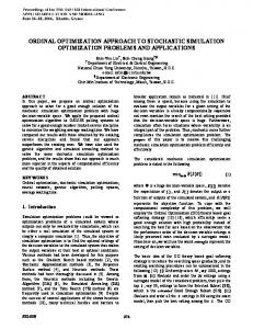
After initializing a maintenance work order (W/O), materials needed as well as manpower requirements of each craft type are listed down. Naturally, some W/Os need more than one craft type. Next, the maintenance cost is estimated and the originator’s approval is obtained before starting the job. Subsequently, the W/O is prioritized and scheduled, first on a weekly basis and then more specifically on a daily basis. Work is started on each W/O as soon as materials and the approval to start are received. The maintenance employees can work for a maximum of 12 hours per day (from 6:00 a.m. to 6:00 p.m.). After finishing the work, a report is sent to the originator for either comment or approval in order to close the W/O. A simplified flowchart of the system is shown in Fig. 1. From the preceding description, each W/O must pass through one of the following phases: 1. Hold (HLD) phase: W/O waiting to receive the materials or approval to start 2. Work (WRK) phase: W/O being processed and undergoing maintenance work
3. The Maintenance Work Order Process The Pipelines Maintenance Unit is concerned with the execution of day-to-day operational and breakdown maintenance jobs. This unit is responsible for scheduled and 2
Figure 1. Simplified flowchart of the maintenance W/O process. Table 2 Service Time Distributions and Statistics for Craft Types
3. Finish (FIN) phase: W/O completed, but waiting for approval to close 4. Close (CLS) phase: W/O completed, approved, and entered into the database.
Craft type
4. Data Collection and Analysis Several entity data had to be collected for the model. The data obtained covered a period of seven months. The data was available with the planner in the Planning Unit but needed several steps of processing. First, the opening dates for W/Os during the stated period were collected. Next, the dates were converted into hours and arranged in increasing order. Finally, the differences between successive opening times were calculated to obtain inter-arrival times in hours for each entity. For each work order opened, the closing date (if applicable), the actual work time in hours, and the number of employees from each craft that worked on the W/O were also recorded. In order to identify the appropriate probability distributions, the data were plotted and the relevant statistics were calculated. To test fitted distributions, the chi-square goodness-of-fit test was used with a level of significance equal to 0.05. The probability distribution for the interarrival time was found to be EXPON (9.79). The remaining results are summarized in Table 2, which shows the probability distributions for the service times (time spent on each work order) for each of the five craft types. For each craft, Table 2 also shows the average number of employees required on each work order, and the service time distributions and statistics.
No. of Avg. no. of Probability Service time men men of craft probability available needed (%) distribution (hours)
AC
2
1.3
18.5
WEIBL (0.83, 19.03)
DG
6
1.49
24.9
WEIBL (0.76, 22.77)
EL
5
1.59
21.3
LOGNR (2.48, 1.07)
MA
3
1.35
23.1
EXPON (13.78)
ME
3
1.11
12.2
WEIBL (0.89, 37.92)
5. Simulation Objectives and Assumptions Before describing the simulation model, its objective and assumptions must be stated. The main performance measure for the Pipelines Maintenance Unit is the average throughput time of W/Os under each craft. Thus, the primary objective is to minimize this average by modifying the work schedules of maintenance employees. Specifically, the aim is to find the optimum days-off schedule of maintenance employees for each craft. Simulation is used for this purpose because of the stochastic nature of maintenance 3
Figure 2. AweSim! network representation of the 5/2 days-off schedule.
workload variation and the complex interaction among several factors.
6. Modelling and Simulation In the programming stage, AweSim! simulation software developed by Symix Systems, Inc. [14] was used. The program was run for 210 simulated days (7 work months), which is well into steady state. During each run, the Create node creates entities (work orders) that pass through the four W/O phases (HLD, WRK, FIN, and CLS). Entities that pass through the WRK node are also distributed to the five craft types (AC, DG, EL, MA, and ME) according to their corresponding probabilities. At the craft type stage, entities (W/Os) wait in the Await node for resources (craft technicians) to start serving them, as soon as these resources finish serving previous entities, and are freed by the Free node. After completing service, Collect node collects the throughput time for each entity. Finally, these entities exit from the system by the Terminate node. It was previously noted that maintenance technicians work according to three different schedules. As shown in Table 1, the Maintenance Unit currently has 13 technicians (1 AC, 6 DG, 3 EL, 1 MA, and 2 ME) on the 5/2 days-off schedule. These technicians work for five days per week from Saturday to Wednesday (it should be noted that the local weekend is Thursday and Friday). On Saturday, the technicians work eight hours from 10:00 a.m. to 6:00 p.m. Then, they work eleven hours per day from Sunday up to Tuesday. On Wednesday, they work five hours from 6:00 a.m. to 11:00 a.m. After that, they are off until 10:00 a.m. on Saturday. As Fig. 2 shows, an Alter node is used to simulate this schedule. Currently, four technicians (one AC, one EL, and two MA) are assigned to the 14/7 days-off schedule. These employees work 14 consecutive days and then take a break for 7 days before they start again, as illustrated in Fig. 3. The third scheduling option is the 7/3–7/4 days-off schedule, which has a sequence of seven workdays followed by three off days, and then seven workdays followed by
5.1 Assumptions • The number of required technicians of each craft varies from one W/O to another. In the model, the number of technicians from each craft type assigned to W/Os was calculated from empirical probability distributions. • No W/Os are in progress at the beginning of the simulation period, that is, only W/Os that are initialized within this period were considered. • Some W/Os need more than one craft type. Historical data was used to determine the percentage of time each craft was needed by a given W/O. • Maintenance craft employees work at an average pace during their work times. • Maintenance employees are fully available during the simulation period, that is, no regular or emergency vacations are taken. 5.2 Definitions • Entity: maintenance work order • Creation time: opening date of the work order • Service time: the actual work time (number of hours) for each craft type on the W/O • Servers: the maintenance craft employees assigned to work on each W/O, that is, the AC, DG, EL, MA, and ME technicians • Waiting time: the time from opening the W/O up to starting work on it by the maintenance employees, including the time needed for the materials to be received or the manager’s approval to be obtained. 4
Figure 3. AweSim! network representation of the 14/7 days-off schedule.
Figure 4. AweSim! network representation of the 7/3-7/4 days-off schedule. four off days. Only two technicians (1 EL and 1 ME) are currently assigned to this schedule, as shown in Fig. 4.
tion runs with different random number seeds, that allows the desired information to be obtained within acceptable accuracy. The confidence interval approach was used to determine this number as follows. First, the confidence intervals for average throughput time were found for successively increasing sample sizes, and then the sample size with the smallest common interval was chosen. Using this approach, the number of replications was determined to be 10. Thus, using 10 simulation runs gives the required information (throughput time of AC craft W/Os) within the desired accuracy.
6.1 Verification and Validation The model was run for a period of seven simulated months, or 210 workdays. In order to validate the model, actual and simulation output values had to be compared. The comparison is based on the throughput time in hours for the W/Os. This was done by running the program five times, with five replications per run, and then taking the average of each run. Five actual system observations were also collected and the difference between each system observation and each simulation run average was found. Finally, the 95% confidence interval of the difference (error) was determined to be [−1.67, 2.52]. Because this interval contains zero, the simulation model can be accepted as a valid representation of the real system. The comparison is illustrated in Table 3 for the AC craft.
6.3 Current System Performance The output obtained from the simulation runs gives much information about the current system performance, such as the number of completed W/Os for each craft type, average waiting time of W/Os for each craft type, average number of orders waiting to be served, and average utilization of workers. However, the main performance measure is the average W/O throughput time for each craft, which is illustrated in Table 4.
Table 3 AC Craft W/Os Simulation Output and Actual Throughput Time (Hours)
Table 4 Current W/O Throughput Time for Each Craft (Hours)
5-run Simulation Actual Difference statistic output observation Mean
7.52
7.1
0.42
Std. dev.
1.22
0.96
1.69
Craft type Average Stand. 95% Confidence dev. interval
6.2 Number of Replications An important aspect of the experimental design is the minimum number of replications, or the number of simula5
AC
9.07
2.24
[7.77, 10.37]
DG
16.85
1.70
[15.86, 17.84]
EL
7.47
1.43
[6.64, 8.3]
MA
24.43
3.29
[22.53, 26.33]
ME
9.14
2.65
[7.61, 10.68]
work order throughput times for all crafts are summarized in Table 6. The reductions in throughput times range from 4% to 67%, with an average of 25%.
7. Alternative Days-Off Schedules 7.1 Machinist (MA) Craft
Table 6 Summary of Best Days-Off Schedules for All Crafts
Looking at the average throughput time for each craft shown in Table 4, it is obvious that the throughput time is higher for the machinist (MA) craft than all the other four crafts. Therefore, alternative days-off schedules were tried for the MA technicians, in order to reduce MA craft W/O throughput time without increasing the number of MA craftsmen. Currently, pipelines maintenance has three MA technicians on two days-off schedules (one on 5/2, two on 14/7). Keeping the number of MA technicians as three, but considering all their possible assignments to the three feasible days-off schedules, there are 10 possible scheduling scenarios (alternatives) shown in Table 5 (alternative 10 is the current schedule). For each scenario, the model was modified according to that scenario and then run again for 10 replications. The new average throughput time for the MA craft W/Os under each scenario is shown in Table 5.
Craft 5/2 14/7 7/3-7/4 From To % (hr) (hr) Reduction
Alternative No. assigned to Ave. throughput number days-off schedules time (hrs) 5/2 14/7 7/3-7/4 3
2
43.58 23.14
1
4
1
1
5
2
1
20.41
1
23.6
6
2
1
24.54
7
1
2
24.39
2
24.33
3
37.22
1
9 1
9.07
8.71
DG
1
EL
2
3
16.85
5.57
66.9
2
2
1
7.47
7.44
0.39
MA
1
1
1
24.43 20.41
16.4
ME
1
1
1
9.14
5.59
4
38.8
8. Conclusion
3 2
10
1
30.68
3
8
1
The highest reduction in throughput time is achieved for the DG craft, for two reasons. First, the DG craft has the largest number (six) of technicians, and thus the greatest number of alternative schedules (27). The second reason is that the original assignment of all six DG technicians to one schedule (5/2) was very inefficient and thus created the highest potential for improvement. On the other hand, the saving in throughput time was lowest for the AC craft, as it has the smallest number (two) of technicians and thus the fewest alternative schedules (6).
Table 5 Days-Off Scheduling Alternatives for 3 MA Technicians
1
AC
2
A simulation-based approach for stochastic workforce daysoff scheduling has been presented. This approach has been applied to an actual days-off scheduling problem involving a pipelines maintenance workforce, consisting of five types of crafts. The best assignment of employees of each craft type to three alternative days-off schedules has been determined. The resulting savings in work order throughput time averaged 25%. These savings are obtained simply by altering the days-off scheduling assignments, without any increase in the number or the cost of maintenance employees. The methodology outlined in this paper is a step in using simulation in solving stochastic employee daysoff scheduling problems. This methodology is applicable to numerous employee scheduling contexts in which the daily labour demands are stochastic, such as maintenance shops, emergency rooms, and call centres. Although the methodology addresses the days-off scheduling problem, it can be easily generalized to the shift scheduling problem. However, application to the tour scheduling problem is not practical because the number of alternative tour schedules tends to be excessively large. Other possible extensions include considering different staffing levels and different off days for each days-off schedule.
24.43
As can be seen from Table 5, scenario number 4 (one person on each of the three days-off schedules) is the best. Under this scenario, the average throughput time for MA work orders will be reduced by 16.4% from 24.43 hours to 20.41 hours. The hiring cost will not change as the pay is the same for all three days-off schedules. 7.2 Remaining Crafts Next, the aim was to find the best days-off schedule for the remaining crafts as was done for the MA craft. Following the same procedure, the best days-off schedules were determined for AC, DG, EL, and ME technicians. The most efficient days-off schedules and corresponding reductions in
Acknowledgment The author is grateful for the research support and facilities provided by King Fahd University of Petroleum and Minerals. 6
References
[12] A.J. Mason, D.M. Ryan, & D.M. Panton, (1998), Integrated simulation, heuristic and optimization approaches to staff scheduling, Operations Research, 46(2), 1998, 161–175. [13] L.D. Smith, Staffing geographically distributed service facilities with itinerant personnel, Computers & Operations Research, 29(14), 2002, 2023–2041. [14] Symix Systems, Inc., AweSim! Version 3.0, Student Version, 1999.
[1] G. Fellers, Use of GPSS/PC to establish manning levels of a proposed just-in-time production facility, Computers & Industrial Engineering, 11(1–4), 1986, 382–384. [2] J.S. Burton, A. Banerjee, & C. Sylla, A simulation study of sequencing and maintenance decisions in a dynamic job shop, Computers & Industrial Engineering, 17(1–4), 1989, 447–452. [3] J.K. Cochran, D.E. Chu, & M.D. Chu, Optimal staffing for cyclically scheduled processes, International Journal of Production Research, 35(12), 1997, 3393–3403. [4] D.J. Davis & V.A. Mabert, Order dispatching and labor assignment in cellular manufacturing systems, Decision Sciences, 31(4), 2000, 745–771. [5] K.K. Yang, S. Webster, & R.A. Ruben, An evaluation of flexible workday policies in job shops, Decision Sciences, 33(2), 2002, 223–249. [6] M. Draeger, An emergency department simulation model used to evaluate alternative nurse staffing and patient population scenarios, Proc. IEEE 1992 Winter Simulation Conf., 1992, 1057–1064. [7] R.S. Dittus, R.W. Klein, D.J. DeBrota, M.A. Dame, & J.F. Fitzgerald, Medical resident work schedules: Design and evaluation by simulation modeling, Management Science, 42(6), 1996, 891–906. [8] M.D. Rossetti, G.F. Trzcinski, & S.A. Syverud, Emergency department simulation and determination of optimal attending physician staffing schedules, Proc. IEEE 1999 Winter Simulation Conf., 1999, 1532–1540. [9] N. Li & L.X. Li, (2000), Modeling staffing flexibility: A case of China, European Journal of Operational Research, 124(2), 2000, 255–266. [10] R. Klungle, Simulation of a claims call center: A success and a failure, Proc. IEEE 1999 Winter Simulation Conf., 1999, 1648–1653. [11] K. Smyllie, Data milling and simulation applied to a staff scheduling problem, High-Performance Computing and Networking, Proceedings, Lecture Notes in Computer Science, 1593, 1999, 1190–1193.
Biography Hesham K Alfares is a professor in the Systems Engineering Department of King Fahd University of Petroleum & Minerals, Dhahran, Saudi Arabia. He obtained his B.Sc degree in electrical and computer engineering from the University of California, Santa Barbara, in 1982; his M.Sc. degree in industrial engineering from the University of Pittsburgh in 1984; and a Ph.D. in industrial engineering from Arizona State University in 1991. His research interests include project and employee scheduling, production and inventory control, petrochemical industry modelling, and maintenance modelling and simulation. He has published 28 papers in these areas in various international journals, in addition to producing many conferences papers, technical reports, and funded research projects.
7