a simulator module for advanced equation assembling - CiteSeerX
Recommend Documents
port equations can be solved. Among these are ... solving complex-valued linear equation systems. For that ... MINIMOS-NT carrier transport can be treated by the drift- diffusion .... the linear combination of these conditions giving an interme- diat
Jan 7, 2017 - for this task. We propose the CM Cloud Simulator to ï¬ll this. gap since it provides a comprehensive and dynamic simulation of. applications with ...
From the Departments of Surgery, Orlando Regional Medical Center, Orlando; ... Hospital, Hollywood; §Tampa General Hospital, Tampa; and the Florida ... includes didactic lectures, group discussion problem-based sessions, and technical skill ... Coll
Nokia Research Center, P.O.Box 45, FIN-00045 Nokia Group, FINLAND tel: +358-9-4376 6427, ... UMTS the need for an advanced radio network simulator will further ..... simulated, it is assumed that there is only one packet call per session.
Assembling the CIA Module: Coalitional Play Fighting in Forager Societies. Michelle Scalise Sugiyama1,2,3, Marcela Mendoza1,2, Frances J. White1,2, and ...
1 Introduction. Semiconductor devices have become an ubiquitous commodity and users have come to expect a constant increase of device performance at ...
E.D.F. research center. 1, av. du G°' De Gaulle, ... calculus is reduced to a single rule, we call the Qualitative Gauss rule. The Qualitative .... device is considered here as linking internal physical variables to boundary physical pa- rameters.
stress paths. The knowledge of learning and teaching styles in engineering education are considered in this research. The software includes a large database of ...
Advanced Simulator Data Mining for Operators' Performance Assessment 3 ... tions and group process for the particular scenario, i.e. accident context on.
Nov 11, 2003 - 2.2 Register a New Module with the GUI Node Editor. ...... module name registration, start-time parameter registration, and run-time get/set.
This paper presents an advanced leg module developed for. HRP-2. HRP-2 is a new humanoid robotics platform, which we have been developing in phase two ...
both in terms of code size and the likelihood of typing errors. ... Generate blocks, like regular and array instantiations, exist within a module definition but outside ...
FloEFD Advanced Module www.3hti.com. D A T A S H E E T. MECHANICAL
ANALYSIS. Concurrent CFD. Mentor Graphics' Mechanical Analysis Division has
...
contiguous data segments to be instantiated in a single statement. ... The array indexes (top_index and bottom_index above) must be known values at compile ...
Assembling History: Achieving Coherent Experiences with Diverse Technologies ... This proliferation of interaction devices and information displays ... coherent experience, our work is also informed by several key issues in the design of public ...
Jul 19, 1990 - A concurrent object is a data structure shared by concurrent .... in a list of events, and then calls analyze (see below) with this ... SeqObj and gets a response value result. 0 ... of these objects need to include two functions, Init
that can occur in saline materials is the migration of brine inclusions through ... State variables (also called unknowns in the text) are: solid velocity, u ..... Several types of formulation have been compared by Galarza et al. ... where the subscr
simulation algorithm corrects the values of the free variables for a given heat rate and total power to pre-malfunction values. In order to demonstrate the reliability ...
3. detailed intra-cellular model and cell-cell interaction, such as diffusion and ligand-receptor .... Decapentaplegic (Dpp), a Drosophila member of the TGF-β family of se- ... signals via the Smad proteins Mother against dpp (Mad) and Medea (Med)11
AbstractâIn the paper, an overview of the current trends in the development of advanced IC packages will be pre- sented. It will be shown how switching from ...
After the HTML form is received, its contents are processed automatically, ... The word processor styles (such as heading, normal paragraph, caption and bold).
It has also been demonstrat- ed in post-crash interviews that night driving, prior sleep .... Post delineators are placed in relation to the edge of the road. Table 1.
to support rapid update of the bounding sphere tree for ... update to increase performance to haptic rates. .... Health Care in the Information Age, IOS Press and.
Figure 1: assembly of abc with (right) and without (left) a conformational ..... The running time of MRS depends on the shape of the parse tree of the input (basic).
a simulator module for advanced equation assembling - CiteSeerX
a substitute equation. As these equations are normally not diagonally dominant they have a negative impact on the condition number and are configured to be ...
A SIMULATOR MODULE FOR ADVANCED EQUATION ASSEMBLING Stephan Wagner1 , Tibor Grasser1 , Claus Fischer∗ , and Siegfried Selberherr2 1
Christian-Doppler-Laboratory for TCAD in Microelectronics at the Institute for Microelectronics 2
Institute for Microelectronics Technical University Vienna Gusshausstr. 27–29, A-1040 Vienna, Austria E-mail: [email protected] ∗
Firma Dr. Claus Fischer Gustav Fuhrichweg 24/1, A-2201 Gerasdorf bei Wien, Austria
KEYWORDS Finite Boxes, Linear Equation Systems, Contact Current, Boundary Conditions, Interface Conditions ABSTRACT We present a generally applicable simulator module which provides an advanced equation assembly system. The module has been originally developed for the simulation of semiconductor devices based on the Finite Boxes discretization scheme and is currently used in the general purpose device and circuit simulator M INIMOS -NT. In general, such simulations require the solution of a specific set of nonlinear partial differential equations which are discretized on a grid. Since the resulting nonlinear problem is solved by a damped Newton algorithm the solution of a linear equation system has to be obtained at each step. The module is responsible for assembling these systems and takes several requirements of the simulation process, namely the representation of boundary conditions, physically motivated variable transformation, preelimination and numerical conditioning, into account.
M INIMOS -NT is a general purpose device and circuit simulator that has been developed at the Institute for Microelectronics for twelve years. Besides the basic semiconductor equations (Selberherr 1984), several different types of transport equations can be solved. Among these are the hydrodynamic equations which capture hot-carrier transport (Stratton 1962, Bløtekjær 1970), the lattice heat flow equation to cover thermal effects like self-heating (Wachutka 1990), and the circuit equations to connect single devices to a circuit (Grasser and Selberherr 2001), both electrically and thermally. Furthermore, various interface and boundary conditions are taken care of, which include Ohmic and Schottky contacts, thermionic field emission over and tunneling through various kinds of barriers. This demands a sophisticated system handling the equation assembly, in order to keep the simulator design flexible. To implement such a system, the requirements will be identified and generalized. A crucial aspect is also the requirement of assembling and solving complex-valued linear equation systems. For that reason the module is able to handle both real-valued and complex-valued contributions and systems.
INTRODUCTION
THE ANALYTICAL PROBLEM
The Finite Boxes discretization method is employed in various kinds of numerical tools and simulators for fast and accurate solving of nonlinear partial differential equation (PDE) systems. The discretized problem is then usually solved by damped Newton iterations which require the solution of a linear equation system at each step. The extensibility and effectiveness of any simulator highly depends on the capabilities of its core modules responsible for handling the linear equation systems. We present an advanced equation assembly module successfully coupled to M INIMOS -NT.
In order to analyze the electronic properties of an arbitrary semiconductor structure under all kinds of operating conditions, the effects related to the transport of charge carriers under the influence of external fields must be modeled. In M INIMOS -NT carrier transport can be treated by the driftdiffusion and the hydrodynamic transport models.
Proceedings 15th European Simulation Symposium Alexander Verbraeck, Vlatka Hlupic (Eds.) (c) SCS European Council / SCS Europe BVBA, 2003 ISBN 3-936150-28-1 (book) / 3-936150-29-X (CD)
Both models are based on the semiclassical Boltzmann transport equation which is a time-dependent partial integrodifferential equation in the six-dimensional phase space. By
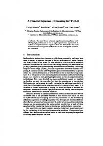
Basically, a device structure can be divided into several segments to enable simulation of advanced heterostructures and to properly account for all conditions (which may cause very abrupt changes) at the contacts and interfaces between these segments, respectively. See Fig. 1 for an illustration of this concept. Every segment represents an independent domain D in one, two, or three dimensions where the PDEs are posed. The equations are implicitly formulated for a quantity x as f(x) = 0 and termed control functions. In order to fully define the mathematical problem, suitable boundary conditions for contacts, interfaces, and external surfaces have to be applied. Generally, such a system cannot be solved analytically, and the solution must be calculated by means of numerical methods. This approach normally consists of three tasks: 1. The domain D is partitioned into a finite number of subdomains Di , in which the solution can be approximated with a desired accuracy. 2. The PDE system is approximated in each of the subdomains by algebraic equations. The unknown functions are approximated by functions with a given structure. Hence, the unknowns of the algebraic equations are approximations of the continuous solutions at discrete grid points in the domain. Thus, generally a large system of nonlinear, algebraic equations is obtained with unknowns comprised of approximations of the unknown functions at discrete points. 3. The third task is to derive a solution of the unknowns of the nonlinear algebraic system. In the best case an exact
0.2um 1.0um
Segment 2 p−Silicon
Interface 2−3
1.0um
The basic semiconductor equations, as given by VanRoosbroeck (VanRoosbroeck 1950), consist of the Poisson equation, the continuity equations for electron and holes as well as the current relations for both carrier types. The unknown quantities of this equation system are the electrostatic potential, ψ, and the electron and hole concentrations, n and p, respectively. C denotes the net concentration of the ionized dopants, ε is the dielectric permittivity of the semiconductor, and R is the net recombination rate. The heat-flow equation and thus the lattice temperature TL is added to account for thermal effects. In the hydrodynamic case the carrier temperatures are allowed to be different from the lattice temperature, adding two more quantities, which are the electron and hole temperatures Tn and Tp .
Segment 1 (Contact) Boundary 1−2
Segment 3 n−Silicon Boundary 3−4
0.2um
the so-called method of moments this equation can be transformed in an infinite series of equations. Keeping only the zero and first order moment equations (with proper closure assumptions) yields the basic semiconductor equations. Considering two additional moments gives the hydrodynamic model (Grasser et al. 2003).
Segment 4 (Contact) 0.6um
Figure 1: Illustration of the segment concept: a simple diode
solution of this system can be obtained, which represents a good approximation of the solution of the analytically formulated problem (which cannot be solved exactly). The quality of the approximation depends on the fineness of the partitioning into subdomains as well as on the suitability of the approximating functions. For the derivation of the discrete problem several methods can be applied. We deal here with point residual methods: the finite difference method based on rectangular grids or the finite boxes (box integration) method allowing general unstructured grids. In the case of orthogonal rectangular grids both methods yield the same discretization. DISCRETIZATION Nonlinear partial differential equations of second order can appear in three variants: elliptic, parabolic, and hyperbolic PDEs. The Poisson equation as well as the steady-state continuity equations form a system of elliptic PDEs, whereas the heat-flow equation is parabolic. To completely determine the solution of an elliptic PDE boundary conditions have to be specified. Since parabolic and hyperbolic PDEs describe
evolutionary processes, time normally is an independent variable and an initial condition is additionally required. Hence, also the transient continuity equations are parabolic. Applying the finite boxes discretization scheme (Selberherr 1984) the equations are integrated over a control volume (subdomain, usually obtained by a Voronoi tesselation) Di which is associated with the grid point Pi . For this grid point a general equation for the quantity x is implicitly given as P =0 (1) fxSi = j Fxi,j + Gi where j runs over all neighboring grid points in the same segment, Fxi,j is the flux between points i and j, and Gi is the source term (see Fig. 2).
1 F 1i
6
F 2i
2
F 6i
i F 3i F 4i
4
Basically, the two (incomplete) equations fxSi and fxSi0 are completed by adding the missing boundary fluxes Fxi,i0 :
Figure 2: Box i with 6 neighbors Grid points on the boundary ∂D are defined as having neighbor grid points in other segments. Thus, (1) does not represent the complete control function fx , since all contributions of fluxes into the contact or the other segment are missing. For that reason, the information for these boxes has to be completed by taking the boundary conditions into account. Common boundary conditions are the Dirichlet condition, which specifies the solution on the boundary ∂D, the Neumann condition, which specifies the normal derivative, and the linear combination of these conditions giving an intermediate type: n · gradx + σx = δ
A method has been under development to implement segment models calculating the interior fluxes and their derivatives independently from the boundary models. The segment models do not have to differentiate the point type, they do not even have to care about the boundary model used. The assembly system is responsible for combining all relevant contributions by using the information given by the boundary models.
To account for complex interface conditions, grid points located at the boundary of the segments (see Fig. 3a) have three values, one for each segment (see Fig. 3b) and a third point located directly at the interface which can be used to formulate more complicated interface conditions like e.g., interface charges. However, to simplify notation these interface values will be omitted in our discussion and only the two interface points, i and i0 , are used.
F 5i
5
Box i
More complex models with exponential interdependency between the solution variables such as thermionic field emission interface conditions (Schroeder 1994, Simlinger 1996) have also been implemented.
Interface Conditions
Gi
3
to differ between interior and boundary points. Considering a general tetrahedron, there exist many kinds of boundary points (depending on the number of edges involved), which have to be treated separately. This leads to a complicated implementation of the models and can make simplifications necessary. Thus, due to organizational and implementational issues this form of coupling should be avoided.
(2)
Generally, the form of these conditions depends on the respective boundary models, and the conditions of which depend on the interior information. For that reason, the equation assembly is often performed in a coupled way, causing complicated modules. For instance, it is absolutely necessary
fxi = fxSi + Fxi,i0 = 0 fxi0 =
fxSi0
− Fxi,i0 = 0
(3) (4)
The intermediate type of interfaces (2) and thus also the two other types of interfaces are generally given in linearized form by: α(xi − βxi0 + γ) = Fxi,i0
(5)
α, β, and γ are linearized coefficients, Fxi,i0 represents the flux over the interface. The three types of interfaces differ in the magnitude of α. In the case of an arbitrary splitting of a homogeneous region into different segments, the boundary models have to ensure that the simulation results remain unchanged. By adding (4) to (3), the box of grid point Pi can be completed and the boundary flux is eliminated. The merged box is now valid for both grid points, for that reason the respective equation can not only be used for grid point Pi , but also for Pi0 .
Whereas the segment models assemble the so-called segment matrix, the interface models are responsible for assembling and configuring the interface system consisting of a boundary and special-purpose transformation matrix. New equations based on (5) can be introduced into the boundary matrix without any limitations on α, thus from 0 (Neumann) to ∞ (Dirichlet). The interface models are also responsible for configuring the transformation matrix to combine the segment and boundary matrix correctly. Depending on the interface type there are two possibilities: • Dirichlet boundaries are characterized by α → ∞. Thus, the implicit equation xi = βxi0 −γ can be used as a substitute equation. As these equations are normally not diagonally dominant they have a negative impact on the condition number and are configured to be preeliminated (see Section ). • For the other types (explicit boundary conditions) the boundary flux is simply added to the segment fluxes. In
Note, that all interface-dependent information is administrated by the respective interface model only. As an additional feature, the transformation matrix can be used to calculate several independent boundary quantities by combining the specific boundary value with the segment entries (also in the case of Dirichlet boundaries). For example, P the dielectric flux over the interface is calculated as i fxSi and introduced as a solution variable because some interface models require the cross-interface electric field strength to determine tunnel processes. Calculation of the normal electric field is thus trivial. Note that this is not the case when ~ n has to be calthe normal component of the electric field E culated using neighboring points when unstructured two- or three-dimensional grids are used. See Fig. 4 for an illustration of these concepts. The transformations are set up to combine the various segment contributions with the boundary system.
the case of a large α, the transformation matrix could be used to scale the entries by 1/α because of the preconditioner used in the solver module.
F 4i’
Box i’
Boundary Conditions Contacts are handled in a similar way to interfaces. However, in the contact segment there is only one variable available for each solution quantity (xC ). Note that contacts are represented by spacial multi-dimensional segments. Furthermore, all fluxes over the boundary are handled as additional solution variables FC (e.g., contact charge QC for Poisson equation, contact electron current InC for the electron continuity equations, or HC as the contact heat flow).
s1
substitute1 = s1
incomplete1 = i1
s2
substitute2 = s2
incomplete2 = i2
Dirichlet b + i1 + i2
boundary = b
zero
m1 + i1
missing1 = m1
incomplete1 = i1
m2 + i2
missing2 = m2
incomplete2 = i2
Other b + i1 + i2
Complete
boundary = b
Boundary + Trans
zero
Segment
Segment 2
Figure 3: Splitting of interface points: Interface points as given in a) are split into three different points having the same geometrical coordinates b)
Figure 4: The complete equations are a combination of the boundary and the segment system. This combination is controlled by the transformation matrix and depends on the interface type.
For explicit boundary conditions one gets fxi = fFC =
fxSi + Fxi,C P FC + i fxSi
=0
(6)
=0
(7)
with i running over all segment grid points. At Schottky contacts explicit boundary conditions apply. The semiconductor contact potential ψs is fixed and given as the difference of the metal quasi-Fermi level (which is specified by the contact voltage ψC ) and the metal workfunction difference potential ψwf . ψs = ψC − ψwf ,
where
ψwf = −
Ew q
(8)
The difference between the conduction band energy EC and the metal workfunction energy gives the workfunction difference energy Ew which is the barrier height of the Schottky contact. For Dirichlet boundary conditions one gets fxi = fFC =
xC − h(xi ) P FC + i fxSi
=0 =0
(9) (10)
with Ci being material parameters. Applying the contact voltage directly to the boundary grid point could cause large arguments of B and hence numerical problems. This is avoided by having a separate variable for the contact voltage. At the beginning of the iteration procedure the constitutive relation for ψC is violated and will only successively be adapted which guarantees numerical stability. The generalized boundary condition is the constitutive relation for the contact potential ψC and reads: fψC = αψC + βIC + γQC − δ = 0
(14)
C where QC is the contact charge and IC = InC + IpC + ∂Q ∂t the contact current. It should be noted that all these quantities are solution variables which are directly available.
SOLVING OF THE NONLINEAR SYSTEM M INIMOS -NT organizes the solving of the nonlinear, but discretized control functions f = 0 using a damped Newton algorithm (k is the number of the iteration step) (Selberherr 1984): Jk · xk+1
=
f (vk )
(15)
k+1
=
(16)
J
=
vk + Fd xk+1 ∂f − ∂v
Here, xC is the boundary value of the quantity, which is a solution variable, whereas (10) is used as constitutive relation for the actual flow over the boundary FC . For example, at Ohmic contacts simple Dirichlet boundary conditions apply. The contact potential ψs , the carrier contact concentrations ns and ps , and in the hydrodynamic simulation case, the contact carrier temperatures Tn and Tp are fixed. The metal quasi-Fermi level (which is specified by the contact voltage ψC ) is equal to the semiconductor quasi-Fermi level. With the constant built-in potential ψbi (calculated after (Fischer 1994)), the contact potential at the semiconductor boundary reads ψs = ψC + ψbi . (11)
where J is the Jacobian matrix, f (v) the residual and x the update or correction vector (solution vector of the linear system) that is then used to calculate the next solution vector v of the Newton approximation.
For Neumann boundaries the flux over the boundary is zero hence the equation assembled by the segment model is already complete.
THE ASSEMBLY MODULE
v
(17)
To avoid overshoot of the solution several damping schemes suggested by Deuflhard (Deuflhard 1974) or Bank and Rose (Bank and Rose 1981) are providing a damping factor Fd . For each Newton iteration step a linear equation system A · x = b has to be assembled and solved.
M INIMOS -NT consists of two separate modules responsible for assembling and solving linear equation systems: Separate Contact Variables Having a separate solution variable for the contact voltage avoids numerical problems with large arguments of the Bernoulli function B. Using a Scharfetter-Gummel discretization scheme (Scharfetter and Gummel 1969) the expression for the current between two grid points i and j reads
1. the assembly module which is directly accessed by the implemented physical models of the simulator, provides an effective application programming interface, various transformation algorithms and the preelimination system. In addition, sorting and scaling plug-ins can be called.
Ii,j = C1 (B(∆)nj − B(−∆)ni ) x with ∆ = C2 (ψj − ψi ) + C3
2. the solver module which is plugged into the assembly module, is responsible for solving the so-called inner linear equation system. The module currently used
(12) (13)
provides a direct (Gaussian) method and two iterative solver schemes. The key demands on the assembly module (class) can be summarized as follows: 1. Application Programming Interface providing methods for • adding contributions to the segment system • adding contributions to the boundary system • adding contributions to the transformation matrix • deleting equations • setting elimination flags • administration of priority information 2. Row transformation: linear combination of rows to extinguish large entries (see Section ). 3. Variable transformation: reduce the coupling of the semiconductor equations (see Section ). 4. Preelimination: eliminate problematic equations by Gaussian elimination to improve the condition of the inner system matrix (see Section ) 5. Call of specific plug-ins (see Section ) for • Scaling: Since a threshold value (tolerance) is used to decide whether to keep or skip an entry, the preconditioner used (Incomplete-LU factorization) requires a system matrix having entries of the same order of magnitude. • Sorting: Reduction of the bandwidth of a matrix to reduce the fill-in. • Solving: Calculate the solution vector of the linear equation system. The input of the assembly module are the contributions of the various segment and boundary models implemented in the simulator. The assembly module compiles these values to a linear equation system, which is subsequently transformed in order to improve the condition of the system matrix.
A plug-in concept has been implemented for scaling, sorting and solving the inner linear equation system, making it possible to adapt or replace these modules easily. The sorting and scaling modules get the system matrix on input and return the sorting and scaling (diagonal) matrices which are then applied by the assembly module. The solver module gets the system matrix and all RHS vectors on input and returns the solution vectors of all inner linear equation systems on output. After reverting all transformations and backsubstituting the preeliminated equations, the output of the assembly module are the complete solution vector (or vectors in case of multiple right-hand-side vectors). In addition, the right-hand-side vector(s) are returned which can be used for various norm calculations. A schematic overview of the complete concept is given in Fig. 5. In the upper left corner the Newton iteration control function IterateOnce is represented, which is divided into two stages and uses an interface class to access the assembly module. Following the solid lines beginning at the interface, the four matrices Tb , As , Ab , and Tv (see Section ) are assembled by using a specific storage class. All diagonal elements are stored in one array, and the off-diagonals, the positions of which are not known in advance, in a balanced binary tree for each row, sorted by column. This allows flexible adding of all entries of the sparse matrices. These structures are then converted to the Modified Sparse Compressed Row (MCSR) format (Saad 1990) and are compiled resulting in the complete linear system (auxFLG), which is preeliminated to get the inner and the outer linear equation system. The inner one (represented by C) is passed to the sorting and scaling plug-ins and finally solved by the solver module. After the solution has been calculated, scaling and sorting have to be reversed and the preeliminated equations are solved back. The Newton adjustment levels (dashed lines) reuse already existing MCSR structures, which reduces the assembling effort: the balanced trees may be skipped completely, and during compiling and preelimination much simpler functions (bold boxes) can be used than in the conventional assembly mode (bold boxes with slash). Assembly of the Complete Linear Equation System
For some simulations, for example derivation of the complex-valued admittance matrix, several linear equation systems differ only in the right-hand-side vector. Thus, the effort for assembling, compiling, preeliminating, sorting, scaling and factorizing of the system matrix actually has to be done only once - and this factored matrix could then be used for all RHS-vectors. For that reason the module is able to simultaneously assemble several RHS vectors.
The semiconductor device is divided into several segments that are geometrical regions employing a distinct set of models. The implementation of each model is completely independent from other models and each model is basically allowed to enter its contributions to the linear equation system. All boundary and interface issues are completely separated
IterateOnce
Interface
Stage1
Tv
Update
Tb
Stage2 Ab
Balanced Tree Assembly
As
Solve Converting To MCSR Clean−Up
Plug−Ins Solve
Scale
Sort
mcsrTv
mcsrAb
mcsrAs
mcsrTb
Compiling Preelimination C auxMR auxFLB auxFLO / auxFLE auxFLG
Figure 5: Schematic assembly overview
from the general segment models, which is represented by assembly structures for the boundary system which are independent from the segment ones. Thus, the system matrix A (the Jacobian matrix in Newton approximation) will be assembled from two parts, namely the direct part Ab (boundary models) and the transformed part As (segment models). The latter is multiplied by the row transformation matrix Tb from the left before contributing to the system matrix A. The right hand side vector b is treated the same way: A = A b + T b · As b = b b + Tb · bs A·x=b
(18) (19) (20)
Although in principle every model is allowed to add entries to all components, the assembly module checks two prerequisites before actually entering the value: first, the quantity the value belongs to is marked to be solved (the user may request only a subset of all provided models) and secondly the priority of the model is high enough to modify the row transformation properties. As stated before, the row transformation is used to complete missing fluxes in boundary boxes. Since a grid point can be part of more than two segments, a ranking using a priority has been introduced. For example, contact models have usually the highest priority and thus their contributions are always used for completion. All three
matrices Ab , As , and Tb and the two vectors bb and bs may be assembled simultaneously, so no assembly sequence must be adhered to. In addition, a forth matrix Tv is assembled which contains information for an additional variable transformation (see Section ). During the assembling process, all contributions are added to values stored in balanced binary trees. After the assembly is finished, these trees are converted to the sparse matrix format MCSR since all necessary mathematical operations are defined for these structures. The analogous, column oriented MCSC format is used to speed up column deleting required by the transformation matrix. During the Newton iterations the structural configuration of these matrices is not modified very often (e.g., on enabling more derivatives), thus, the tree assembly may be skipped and the variables may be entered directly in the already existing MCSR structures. Hence, the effort for deleting, tree assembling, reallocating and converting can be saved which drastically speeds up the assembly process. However, if an entry in the structure is missing, the conventional assembly procedure can be easily restarted. The so-called Newton adjustment addresses not only the assembly matrices, but also the resulting structures of the compilation and preelimination process.
The Complete Linear System
Row Transformation The complete linear equation system is built from an original system (segment system), which is the main matrix As and the main right hand side vector bs , both of them representing cumulated fluxes and their derivatives to the system variables. Basically, the fluxes are calculated from segment models which are the models for the interior of discretized regions. The matrix is a linear superposition of very small matrices, one for each flux, with a few non-zero elements only. Consequently, the same superposition applies for the vector bs . All fluxes are assigned to boxes, a box is in turn assigned to each variable. As the control function for a box is defined by the user, for example being the sum of all fluxes leaving the box, the fluxes leaving the boxes are entered into the vector bs in the places appropriate for the variables that are assigned to the boxes. In context of the Newton method, matrix As contains the negative derivatives of the values in bs to the system variables, so that the change dx in the variables leads to a change −As · dv = dbs in the right hand side. Considering bs a function of the variable vector v, one can write:
The full system is assembled from the segment system and the boundary system in the following way: b = b b + Tb · bs A = A b + T b · As A·x=b (Ab + Tb · As ) · x = bb + Tb · bs
(25) (26) (27) (28)
As stated above, vector x represents a linear change of the variables vector v. With equation (29) and the new variables vector vn from equation (30), the new value bn of the vector function b(v) will be described by the linear approximation in equation (31). x = dv vn = v + x db · dv = b − A · x = 0 bn (vn ) = b + dv
(29) (30) (31)
Variable Transformation bs = bs (v) dbs As = − dv
(21) (22)
The boundary conditions will enforce some special physical conditions at the boundaries. The control functions of boxes along the boundary will usually be completed by the boundary conditions. For example, a Dirichlet boundary condition will use the dielectric flux cumulated in the boundary box to calculate the surface charge on the surface of the adjacent material. The equation used to calculate the value of the boundary variable, however, will not always make use of the fluxes accumulated in the main system. The boundary conditions are therefore implemented by two elements: a boundary system (Ab and bb ) and a transformation matrix Tb . The purpose of the matrix Tb is the forwarding of the fluxes of the main system to their final destination or their resetting if they are not required. The system of Ab and bb represents additional or substitutional parts of the final equation for the variables at the boundaries. Again, the entries in the matrix As are the negative derivatives of the right hand side vector bb to the variable vector v:
bb = bb (v) dbb Ab = − dv
(23) (24)
Especially in the case of mixed quantities in the solution vector, a variable transformation is sometimes helpful to improve the condition of the linear system. The representation chosen here allows to specify fairly arbitrary variable transformations to be applied to the system. Basically, a matrix Tv is assembled and multiplied with the system matrix. For example, to reduce the coupling of the semiconductor equations and thus improve the condition of the system matrix, a transformation of the stationary drift-diffusion model is suggested in (Ascher et al. 1986). The transformation expressed by matrix Tv is given by equation (32): ((Ab + Tb · As ) · Tv ) · (T−1 v · x) = = (bb + Tb · bs )
(32)
For compactness the following substitutions will be used hereinafter: ˜ = ((Ab + Tb · As ) · Tv ) A (T−1 v
˜= x · x) ˜ = (bb + Tb · bs ) b
(33) (34) (35)
Preelimination The main matrix As consists of fluxes that will (if the control functions are correctly assigned to the variables) satisfy
the criterion of diagonal-dominance that is necessary to make the linear equation system solvable with an iterative solver. The transformations and additional terms imposed by the boundary conditions may heavily disrupt this feature both in structural and numerical aspects. Some of the boundary or interface conditions can make the full system matrix so illconditioned that this simply prevents iterative linear solvers from converging. One solution to this problem which occurs only at the boundary variables that are affected in this way by the boundary conditions, is to apply Gaussian elimination to these variables/equations before the system is passed on to the linear solver. After the iterative solver has converged, the eliminated variables are calculated by backsubstitution into the eliminated equations. Before they can be eliminated, the equations of this type are sorted to the back of the matrix, together with their assigned variables. This is done by applying a permutation matrix P to the linear equation system. The permutation matrix is calculated automatically on solving the system. The equation causing a possibly ill condition have to be marked for preelimination. The outer system is removed from the linear equation system and later solved by Gaussian elimination, the inner system is passed on to an iterative solver. See Fig. 6 (Fischer 1994) for an illustration of this concept.
the row/column index that narrows the section passed to the linear solver is a strict unity matrix. Call of Specific Plug-Ins Matrices arising from the discretization of differential operators are sparse, because only neighbor points are considered. To reduce memory consumption, only the non-zero elements are stored (see MCSR format). During a factorization of A into an upper and lower triangular matrix A = L · U, additional matrix elements termed fill-in (Selberherr 1984) become non-zero and require additional memory. In order to minimize the fill-in, the system matrix is usually sorted. The standard module provided by default obtains the sorting matrix Rs (similar to P) by a Cuthill-McKee-based algorithm. To provide the (ILU-) preconditioner with a normalized representation of the matrix, a scaling of all values has to be performed. The standard algorithm used by default works with a two-stage strategy (Fischer and Selberherr 1994): In the first stage, the matrix is scaled such that the diagonal elements are one. The second stage attempts to suppress the off-diagonals while keeping the diagonals at unity. The resulting scaling matrices Sr and Sc are diagonal matrices, and −1 RT s equals Rs . With Ai · xi = bi as the inner system, the effect of sorting and scaling is given in (37): T −1 (Sr · (RT s · Ai · Rs ) · Sc ) · (Sc · (Rs · xi )) =
= Sr · (RT s · bi )
The resulting system is given by (36): ˜ ˜ · PT ) · (P · x ˜ ) = (E · P · b) (E · P · A
(36)
Here, P is the permutation matrix with its inverse equal to its transposed matrix PT . E is a matrix of elimination coefficients obtained as the lower matrix L of a Gaussian elimination of the permuted system matrix. E contains non-zero off-diagonals in the outer parts only, the inner matrix up to
Permutation Vector
System Matrix
*
(37)
The assembly module is finally responsible for passing the inner linear equation system to the solver module. There are several approaches to obtain the solution vector: a Gaussian solver factorizes the matrix with a complete LU factorization, followed by a forward- and a backward substitution. Iterative solvers use successive approximations of this vector to obtain more accurate solutions to a linear equation system at each step (Barrett et al. 1994). In addition, the solver module provides a general interface to alternative solvers. After returning from the solver module, scaling and sorting are reverted and the preeliminated equations are backsubstituted. CONCLUSION
Row Index
Inner Matrix
* Outer Matrix *
Figure 6: All equations marked for preelimination (*) are moved to the outer system matrix, the others remain in the inner one.
We presented the concept and implementation of an advanced assembly module successfully applied in the device and circuit simulator M INIMOS -NT. The generally applicable module provides all conceptional and numerical features required for assembling and solving linear systems arising from discretized PDEs. The presented concepts result in superior stability of M INIMOS -NT without restricting model implementation and further development. The general approach for treating boundary conditions yields in combination with several preconditioning measures diagonaldominant linear equation systems well prepared for advanced
solver algorithms. As a result, boundary conditions for specific operating points can be directly applied without stepping to the desired value as is very common even in commercial simulators. AUTHOR BIOGRAPHIES STEPHAN WAGNER was born in Vienna, Austria, in 1976. He studied electrical engineering at the Technical University Vienna, where he received the master degree of ”Diplomingenieur” in 2001. As a member of the M INIMOS -NT development group he joined the Institute for Microelectronics in November 2001, where he is currently working on his doctoral degree. His scientific interests include device and circuit simulation, numerical aspects and software technology. TIBOR GRASSER was born in Vienna, Austria, in 1970. He studied communications engineering at the Technische Universit¨at Wien where he received the ‘Diplomingenieur’ and the doctoral degree in technical sciences in 1995 and 1999, respectively. He joined the Institut f¨ur Mikroelektronik in April 1996 where he is currently employed as an Assistant. In 2002 he received the venia docendi on Microelectronics. Since 1997 he has been heading the MINIMOS-NT development group, working on the successor of the highly successful MINIMOS program. CLAUS FISCHER Claus Fischer was born in Vienna, Austria, in 1967. He received the doctoral degree in technical sciences from the ’Technische Universit¨at Wien’ in 1994. He started the Minimos NT project in order to extend the proven concepts and numerical methods of Minimos to complex geometrical and topological structures and introduced a generalized physical interface treatment. After Ph.D., he worked in the semiconductor industry for three years. He now runs his own software engineering company in Austria. His interests cover a range of software engineering topics for industrial use, from technical to business applications. SIEGFRIED SELBERHERR was born in Klosterneuburg, Austria, in 1955. He received the degree of ‘Diplomingenieur’ in electrical engineering and the doctoral degree in technical sciences from the ‘Technische Universit¨at Wien’ in 1978 and 1981, respectively. Dr. Selberherr has been holding the ‘venia docendi’ on ‘Computer-Aided Design’ since 1984. Since 1988 he has been the head of the ‘Institut fu¨ r Mikroelektronik’ and since 1999 he has been dean of the ‘Fakult¨at f¨ur Elektrotechnik’. His current topics are modeling and simulation of problems for microelectronics engineering. REFERENCES Ascher, U.; P.A. Markowich; C. Schmeiser; H. Steinru¨ ck; and R. Weiss. 1986. Conditioning of the Steady State Semiconduc-
tor Device Problem. Technical Report 86-18, University of British Columbia. Bank, R.E. and D.J. Rose. 1981. ”Global Approximate Newton Methods”. Numer.Math., 37:279–295. Barrett, R.; M. Berry T.F. Chan; J. Demmel; J. Donato; J. Dongarra; V. Eijkhout; R. Pozo; C. Romine; and H. Van der Vorst. 1994. Templates for the Solution of Linear Systems: Building Blocks of Iterative Methods. SIAM, Philadelphia, PA. Bløtekjær, K. 1970. ”Transport Equations for Electrons in TwoValley Semiconductors”. IEEE Trans.Electron Devices, ED17(1):38–47. Deuflhard, P. 1974. ”A Modified Newton Method for the Solution of Ill-Conditioned Systems of Nonlinear Equations with Application to Multiple Shooting”. Numer.Math., 22:289–315. Fischer, C. 1994. Bauelementsimulation in einer computergest¨utzten Entwurfsumgebung. Dissertation, Technische Universit¨at Wien. http://www.iue.tuwien.ac.at. Fischer, C. and S. Selberherr. 1994. ”Optimum Scaling of NonSymmetric Jacobian Matrices for Threshold Pivoting Preconditioners”. In Intl. Workshop on Numerical Modeling of Processes and Devices for Integrated Circuits NUPAD V, pages 123–126, Honolulu. Grasser, T.; H. Kosina; M. Gritsch; and S. Selberherr, 2001. ”Using Six Moments of Boltzmann’s Transport Equation for Device Simulation”. J.Appl.Phys., 90(5):2389–2396. Grasser, T.; T.-w. Tang; H. Kosina; and S. Selberherr. 2003. ”A Review of Hydrodynamic and Energy-Transport Models for Semiconductor Device Simulation”. Proc.IEEE, 91(2):251–274. Grasser, T. and S. Selberherr. 2001. ”Fully-Coupled ElectroThermal Mixed-Mode Device Simulation of SiGe HBT Circuits”. IEEE Trans.Electron Devices, 48(7):1421–1427. Saad, Y. 1990. A Basic Tool Kit for Sparse Matrix Computations. Technical Report, RIACS, NASA Ames Research Center, Moffett Field, CA 94035. Scharfetter, D.L. and H.K. Gummel. 1969. ”Large-Signal Analysis of a Silicon Read Diode Oscillator”. IEEE Trans.Electron Devices, ED-16(1):64–77. Schroeder, D. 1994. Modelling of Interface Carrier Transport for Device Simulation. Springer. Selberherr, S. 1984. Analysis and Simulation of Semiconductor Devices. Springer, Wien–New York. Simlinger, T. 1996. Simulation von HeterostrukturFeldeffekttransistoren. Dissertation, Technische Universit¨at Wien. http://www.iue.tuwien.ac.at. Stratton, R. 1962. ”Diffusion of Hot and Cold Electrons in Semiconductor Barriers”. Physical Review, 126(6):2002–2014. VanRoosbroeck, W.V. 1950. ”Theory of Flow of Electrons and Holes in Germanium and Other Semiconductors”. Bell Syst.Techn.J., 29:560–607. Wachutka, G.K. 1990. ”Rigorous Thermodynamic Treatment of Heat Generation and Conduction in Semiconductor Device Modeling”. IEEE Trans.Computer-Aided Design, 9(11):1141– 1149.