Numerical formulation for a simulator (CODE_BRIGHT) - CiteSeerX

Numerical formulation for a simulator (CODE_BRIGHT) for the coupled analysis of saline media S. Olivella, A. Gens, J. Carrera and E.E. Alonso

Coupled analysis of saline media 87 Received June 1995 Revised October 1995

Universitat Politècnica de Catalunya, Barcelona, Spain Introduction Salt rocks are being considered as potential recipients for geologic disposal of nuclear waste because of their favourable hydraulic and mechanical properties. In essence, processes controlling the behaviour of salt rocks are similar to those occurring in other media, except that they take place at unusually fast rates. The high solubility of salt in water is one of the causes of these high rates. In fact, creep deformation of wet salts takes place much faster than under dry conditions. This can be explained by means of a mechanism of creep deformation based on salt dissolution, molecular diffusion and precipitation at the pore scale caused by stress concentration[1,2]. The high hygroscopic character of salt facilitates condensation of water in the mineral surface which in turn causes dissolution. These phase change processes are associated with release or uptake of energy. Another phenomenon that can occur in saline materials is the migration of brine inclusions through the crystalline structure[3,4]. These inclusions may disappear in grain boundaries or come into existence in contacts where brine films are entrapped. Therefore, porosity may undergo changes caused not only by deformation but also due to dissolution/precipitation or, perhaps with a lesser influence, by brine inclusions production/annihilation. The complex behaviour of saline media requires new theoretical and numerical developments. The study of the basic mechanisms has revealed that coupling between thermal, hydraulic and mechanical problems may be required in some cases. We have developed[5] the governing equations for nonisothermal multiphase flow of brine and gas in deformable saline media. These include mass balance equations for the species in the system (salt, water and This work has been performed under contract with ENRESA (Empresa Nacional de Residuos) in the framework of a project partially funded by the ECC (European Community Commission) (Contract No. FI.2W-CT90-0068). Financial support of the DGICYT through research project PB92-0702 is also acknowledged. The work of the first author has also been supported by the Generalitat de Catalunya (Spain) and the Technical University of Catalunya (UPC, Spain).

Engineering Computations, Vol. 13 No. 7, 1996, pp. 87-112. © MCB University Press, 0264-4401

EC 13,7

air), energy balance equation and stress equilibrium equation. Equilibrium restrictions complete the theoretical formulation. This paper presents a numerical formulation required for solving this complex problem in a practical way. An example of its application is also included.

88

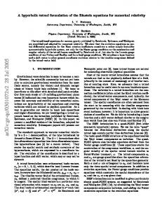
Problem A porous medium composed of salt grains, brine and air will be studied. Crushed fills, manufactured bricks or the host rock are all media that correspond to this composition. Thermal, hydraulic and mechanical aspects should be considered, including coupling between them in all possible directions. As illustrated in Figure 1, the problem is formulated in a multiphase and multispecies approach. The three phases are: (1) solid phase (s): composed of crystalline salt with brine inclusions; (2) liquid phase (l): saturated dissolution of salt in water; air dissolved is also considered; and (3) gas phase (g): mixture of dry air and water vapour. The three species are: (1) salt (h): sodium chloride, as solid or dissolved in the liquid phase; (2) water (w): as liquid in brine or evaporated in the gaseous phase; and (3) air (a): dry air, as gas or dissolved in the liquid phase. The following relevant assumptions and aspects are taken into account in the formulation of the problem.

Brine inclusions

Gas phase (air and water)

Pores

Solid phase (salt and water) Figure 1. Schematic representation of the porous medium composed by salt grains, brine and gas

Grains

Liquid phase (water, salt and air)

• • •

• •

•

•

•

• •

Uniform salt composition. Solubility controlled dissolution /precipitation is the only chemical process taken into account. Fluid inclusions are filled with saturated brine, gas is not allowed in the inclusions. Dry air is considered a single species and is the main component of the gaseous phase. Henry’s law is used to express equilibrium of dissolved air. Thermal equilibrium between phases is assumed. This means that the three phases are at the same temperature. Vapour concentration is in equilibrium with the liquid phase, the psychrometric law expresses its concentration. Correction for the influence of dissolved salt is included because Raoult’s law is not correct for brines. . State variables (also called unknowns in the text) are: solid velocity, u (three spatial directions); liquid pressure, P l ; gas pressure, Pg ; and temperature, T. Though less relevant, mass fraction of water in the solid phase ωws is used when inclusions are considered. Balance of momentum for the medium as a whole is reduced to the equation of stress equilibrium together with a mechanical constitutive model to relate stresses with strains. Strains are defined in terms of displacements. Small strains and small strain rates are assumed for solid deformation. Advective terms due to solid displacement are neglected after the formulation is transformed in terms of material derivatives (in fact, material derivatives are approximated as eulerian time derivatives). In this way, volumetric strain is considered. Balance of momentum for dissolved species and for fluid phases are reduced to constitutive equations (Fick’s law and Darcy’s law). Physical parameters in constitutive laws are a function of salt concentration, among other variables. For example: concentration of vapour under planar surface (in psychrometric law), surface tension (in retention curve), dynamic viscosity (in Darcy’s law), are strongly dependent on salt concentration.

Governing equations The governing equations for non-isothermal multiphase flow of brine and gas through porous deformable saline media are presented by Olivella et al.[5,6]. A detailed derivation is given there, and only a brief description is included in this paper. The equations that govern this problem can be categorized into four main groups. These are: balance equations, constitutive equations, equilibrium relationships and definition constraints. Equations for mass balance were

Coupled analysis of saline media 89

EC 13,7

90

established following the compositional approach. That is, mass balance is performed for water, air and salt species instead of using solid, liquid and gas phases. An equation for balance of energy is established for the medium as a whole. The equation of momentum balance for the porous medium is reduced to that of stress equilibrium. Among the constitutive aspects, we have devoted more attention to the study of the mechanical behaviour of porous salt aggregates because it is a poorly known field. A model which includes creep behaviour has been developed[1,7,8]. This was obtained by building on the theoretical ideas and experimental work carried out by Spiers et al.[2]. Balance equations The compositional approach is adopted to establish the mass balance equations. Volumetric mass of a species in a phase (e.g. salt in liquid phase θ hl ) is the product of the mass fraction of that species ωhl ) and the bulk density of the phase (ρ l ), i.e. θ hl = ω hl ρl. The total mass flux of a species in a phase (e.g. flux of salt present in liquid phase j hl) is, in general, the sum of three terms: •

the non-advective flux: i hl , i.e. diffusive/dispersive;

•

the advective flux caused by fluid motion: θ hl ql, where ql is the Darcy’s flux; and . . the advective flux caused by solid motion: φ Sl θ hl u where u is the vector of solid velocities, Sl is the volumetric fraction of pores occupied by the liquid phase and φ is porosity.

•

The sum of the non-advective and fluid motion advective fluxes is separated from the total flux in order to simplify algebraic equations. This flux is relative to the solid phase and is denoted by j' hl. It corresponds to the total flux minus the advective part caused by solid motion. When solid deformation is negligible, then j' = j. The relative contribution of each flux term to the total flux is not always the same. For instance, diffusion will become more important if advection is small. Mass balance of salt Mass balance of salt present in the medium is written as: (1) where θ hs and θ hl are the mass of salt per unit volume of solid and liquid phase, j hs and j hl are the salt fluxes of salt as present in the solid and liquid phases, respectively, and f h is an external supply of salt. From this equation, an expression for porosity variation was obtained as:

Coupled analysis of saline media (2) where j' hs and j' hi are fluxes with respect to the solid (note that the advective part associated with solid motion has been separated). The material derivative with respect to the solid has been used and its definition is: (3) Equation (2) expresses the variation of porosity caused by processes considered in the salt mass balance. Porosity changes are due to volumetric deformation, dissolution/precipitation and inclusion production/annihilation. The reader may notice that equation (2) reduces to the balance of solid phase if dissolution . and inclusions are not permitted, i.e. Dsφ /Dt = (1–φ) ∇ .u , which expresses the variation of porosity caused only by volumetric deformation. Mass balance of water Water is present in all three phases. The total mass balance of water is expressed as: (4) where fw is an external supply of water. An internal production term is not included because the total mass balance inside the medium is performed. The use of the material derivative (equation 3) leads to:

(5) The final objective is to find the unknowns from the governing equations. Therefore, the dependent variables will have to be related to the unknowns in some way. For example, degree of saturation will be computed using a retention curve which should express it in terms of temperature, liquid pressure and gas pressure.

91

EC 13,7

92

Porosity appears in equation (5) not only as a coefficient, but also in a term involving its variation caused by different processes. It is also hidden in variables that depend on porosity (e.g. intrinsic permeability). The way of expressing the derivative term as a function of the state variables is via the salt mass balance equation (equation 2). This allows the influence of porosity variation to be taken into account correctly in the balance equation for water. It has to be noted that in equation (5) the material derivatives can be approximated as eulerian if the assumption of small strain rate is performed . while the volumetric change (porosity derivative and volumetric strain) ∇ . u is not neglected. This is the classical way of obtaining the coupled flowdeformation equations. Mass balance of air Once the other mass balance equations have been written it is straightforward to obtain the mass balance of air taking into account that air is the main component of the gas phase and that it may be also present as dissolved air in the liquid phase. It is an equation similar to that of water balance, with the exception that air is not allowed in the solid phase (i.e. θ as = 0). This assumption has been adopted because it is rare to find gas in the fluid inclusions[3]. Mass balance of water in inclusions The terms concerning the solid phase in the mass balance of the total water are used to obtain this equation. Since this equation balances a fraction of the water present in the medium, the phase change term is explicit. This specific problem has been studied by Ratigan[9]. The approach presented by this author was adopted for the terms related to inclusion migration. Momentum balance for the medium The momentum balance reduces to the equilibrium of stresses if the inertial terms are neglected: (6) where σ is the stress tensor and b is the vector of body forces. Details of the mechanical constitutive model can be found in[1,6,7]. Internal energy balance for the medium The equation for internal energy balance for the porous medium is established, taking into account the internal energy in each phase: (Es , El , Eg ):

(7)

where ic is energy flux due to conduction through the porous medium, the other fluxes (jEs , jEl , jEg ) are advective fluxes of energy caused by mass motions and f E is an internal/external energy supply. In this case this term accounts, for instance, for energy dissipation due to medium deformation which is not explicit because it is negligible in most cases. The use of the material derivative (equation 3) allows an equation formally similar to equation (5) to be obtained. The reason for the similarity is that both water and internal energy are considered present in the three phases. For space reasons further developments are not included and may be found in[5,6].


Constitutive equations and equilibrium restrictions Associated with this formulation there is a set of necessary constitutive and equilibrium laws. Table I is a summary of the constitutive laws and equilibrium restrictions that should be incorporated in the general formulation. The dependent variables that are computed using each of the laws are also included. Equation

Variable name

Variable

Constitutive equations Darcy’s law Fick’s law Inclusion migration law Fourier’s law Retention curve Mechanical constitutive model Phase density Gases law

Liquid and gas advective flux Vapour and salt non-advective flux Brine inclusions non-advective flux Conductive heat flux Liquid phase degree of saturation Stress tensor Liquid density Gas density

ql , qg i wg, i hl i ws ic Sl σ ρl ρg

Equilibrium restrictions Solubility Henry’s law Psychrometric law

Salt dissolved mass fraction Air dissolved mass fraction Vapour mass fraction

ω hl ω al ω wg

As stated above the governing equations for non-isothermal multiphase flow of brine and gas through porous deformable saline media have been established by Olivella et al.[5]. A detailed derivation is presented there. The theoretical work briefly presented above has been used as a basis for the development of a computer program called CODE_BRIGHT, which stands for COupled DEformation, BRIne, Gas and Heat Transport problems. Numerical approach used in the program CODE_BRIGHT The resulting system of PDEs (partial differential equations) is solved numerically. The numerical approach can be viewed as divided into two parts:

Table I. Constitutive equations and equilibrium restrictions

EC 13,7

94

spatial and temporal discretizations. The finite element method is used for the spatial discretization while finite differences are used for the temporal discretization. The discretization in time is linear and the implicit scheme uses two intermediate points, t k+ε and t k+θ between the initial tk and final t k+1 times. Finally, since the problem presented here is non-linear, the Newton-Raphson method was adopted to find an iterative scheme. Once the salt balance is substituted in the other balance equations, computation of porosity at an intermediate point is not necessary because its variation is expected to occur at slow rates. For this reason, porosity is integrated explicitly, that is, the values at t k are used. Since the variation of porosity is expressed by the salt mass balance equation, this assumption leads also to some advantages for the iterative scheme. After the spatial discretization of the partial differential equations, the residuals that are obtained can be written (for one finite element) as:

(8a) . where r are the residuals, d are the storage or accumulation terms, a are the conductance terms, and b are the sink/source terms and boundary conditions. After time discretization and using a more compact form:

(8b) where k is the time step index, X = ((ux , uy , uz, Pl , Pg, T, ω ws )1, …, (ux, uy, uz, Pl, Pg, T, ωws )n) is the vector of unknowns ( i.e. a maximum of seven degrees of freedom per node), and A represents the conductance matrix. A detailed description of this residual (equation 8) is included in the Appendix. The Newton-Raphson scheme of solution for this non-linear system of AEs is: (9) where l indicates iteration. In the following subsections we will explain in detail how each term is handled in the program CODE_BRIGHT.

General aspects In the present approach, we use the standard Galerkin method but we introduce some variations in order to facilitate computations. General aspects related to numerical solution of hydrogeological problems can be found in[10]. As shown in the previous section, in the mass and energy balance equations the following terms may be distinguished: •

Storage terms. These terms represent the variation of mass or energy content and therefore, they are calculated by means of variables such as degree of saturation, density, porosity, mass fraction and specific energy.

•

Advective fluxes. The advective fluxes caused by motion of fluids are computed using Darcy’s law and, except for the coefficients, they are explicit in terms of pressure gradients.

•

Non-advective fluxes. These terms, computed through Fick’s law, are proportional to gradients of mass fractions which do not belong to the set of unknowns. Fourier’s law is used for the conductive heat flux and it expresses proportionality to temperature gradients.

•

Volumetric strain terms. In fact, these terms are also storage terms. They . are proportional to ∇ . u which is equivalent to the volumetric strain rate.

•

Sink/source terms.

In saline materials, non-linear creep behaviour takes place. This implies that the mechanical problem becomes non-linear. Coupling with hydraulic and thermal problems occurs in different ways (for instance, thermal expansion and thermal dependence of creep parameters). Another difficulty concerning the mechanical problem is related to the behaviour of nearly-incompressible materials. In this regard, element locking appears when analysing creep deformation of rock salts. This difficulty has received the attention of several researchers. A general discussion can be found in[11] while techniques for nonlinear problems can be found in[12]. Solution of the salt balance equation to obtain porosity evolution requires a specific algorithm if porosity is considered a function of time and space but with constant values over each finite element. In order to explain the treatment of the different terms and equations the following notation is introduced: •

node i: node in a finite element mesh.

•

e1, e2, …, em: elements that contain node i, i.e. a cell centred in node i is composed by a fraction of these elements. m is variable from node to node and it is not related to the number of nodes per element (see Figure 2).

•

nem: number of nodes in element em. For example, nem = 3 for triangles, nem = 4 for quadrilaterals, nem= 4 for tetrahedrons, etc.


EC 13,7

e2 e1

96

Cell associated to node i

i em

Figure 2. Representation of a cell in a finite element mesh

• • • • • •

j

(.) k: the quantity is computed at time k of the temporal discretization. The same for k + 1, k + ε or k +θ. (.)em: the quantity is computed in element em. This means at the centre of the element or, in other words, using the average of nodal unknowns. (.) i: the quantity is computed in node i as a function of the unknowns in that node. ( . )i,e m : the quantity is computed in node i but with the material properties corresponding to element em. Vem: volume of element em. ξi: shape function for node i.

Treatment of storage terms In this subsection we refer to terms not related to volumetric strain or porosity variation which are included in subsequent subsections. The storage or accumulation terms are computed in a mass conservative approach[13-15]. The conservative approach dicretizes directly the accumulation terms while the capacitative approach uses the chain rule to transform time derivatives in terms of the unknowns. Milly[15] proposes modifications of the the capacitative approach in order to conserve mass. It seems reasonable that the mass conservative approach should give a more accurate solution than the capacitative approach. Mass conservation in time is achieved if the time derivatives are directly approximated by a finite difference in time. Finite element method for the space discretization conserves mass. This latter affirmation is easily proven by adding up all nodal equations. Flow terms cancel out (due to the definition of the shape functions) and the resulting equation represents mass accumulation in the entire domain. Milly[15] concludes that if mass conservation takes place, only the distribution of moisture in the medium is affected by the discretization

(spatial and temporal) and iteration. In other words, the mass balance is guaranteed independently of discretization and iteration. On the other hand, Celia et al.[14] demonstrate that if the Picard iterative scheme is used the same computational effort is necessary for the conservative and the capacitative approaches. This statement cannot be made if the NewtonRaphson method is used because in such case the conservative approach is much more economical per iteration. Celia et al.[14] also point out that conservation of mass is insufficient to guarantee good numerical solutions and oscillations can also appear. Several types of formulation have been compared by Galarza et al.[16] for the unsaturated flow problem considering seven cases of study. The comparison in terms of pressures indicate a consistently better performance of the capacitative approach for some cases, and similar accuracy in other cases. This is in agreement with the idea that although mass is conserved, the distribution of water in the medium may be not as good as with another scheme. In spite of the latter findings, we have opted for the mass conservative approach because the capacitative method requires computing derivatives of the accumulation time derivatives with respect to unknowns. If the chain rule is used to split the accumulation time derivatives in terms of the unknowns (temperature, liquid pressure and gas pressure), the use of the Newton-Raphson method leads to second derivatives (also crossed, for example with respect to temperature and pressure) of the non-linear terms. This results in a very uneconomical scheme. Since the differences in accuracy are not very strong, the use of a much more economical but slightly less accurate scheme can produce a more powerful approach because a more refined mesh can improve the solution. A typical storage term is (from equation 5) the variation of water in the gas phase: (10) where the material derivative with respect to the solid is approximated as an eulerian derivative because of the small strain rate assumption. The weighted residual method is applied to the governing equations and, for node i, (10) is transformed into:

(11) where ξi is the shape function for node i.


EC 13,7

98

At this point of the development we assume that porosity is defined elementwise. An elementwise variable[17] is space-constant over every element, but different from element to element. We will use φ ekm for porosity in element em at time k. Similarly, a cell-wise variable[17] is space constant over the cell centred in the node. It would be very easy to compute (11) if the time derivative could be computed in a cell-wise way, because one value would be sufficient for node i and (11) would be transformed into a very simplified form. However, the degree of saturation is not only a function of nodal unknowns but also of material properties such as porosity or retention parameters. The latter must be defined element-wise (for instance, this is absolutely necessary if a low porosity rock is in contact with a porous medium). To overcome this difficulty, the time derivative in (11) is computed from nodal unknowns but with material properties of every element in contact with the node. Hence m values are necessary in node i. Obviously if part of this time derivative is not material dependent (density and concentration are only function of temperature and pressure) then the corresponding variables are only computed in the node. This leads to a kind of modified cell-wise variables. Making use of these approximations, we finally obtain, for example for any integral in (11): (12) where a simple finite difference is used for the time discretization. This approximation allows us to make the space integration independently of the physical variables. Therefore, computation of geometrical coefficients is necessary only once for a given finite element mesh. The integral of the shape function over an element is equal to V e m /n e m for the case of linear shape functions. These geometrical coefficients are also called influence coefficients[18]. Without loss of generality, they can be computed either analytically or numerically. Finally, it should be pointed out that this formulation gives rise to a concentrated scheme, which means that the storage term in node i is only a function of unknowns in node i. This is clearly advantageous from a computational point of view[10]. Treatment of advective terms The weighted residual method is applied to each balance equation. Then Green’s theorem allows one to reduce the order of the derivatives and the divergence of flows is transformed into two terms, one of them with the gradient of the shape function. Hence, after that, in the water balance equation of node i we find, the following advective term:

Coupled analysis of saline media (13) where the subscript j indicates summation over element nodes. Pg is a nodewise[17] variable, which means that it is defined by its nodal values and interpolated on the elements using the shape functions. Generalized Darcy’s law has been used to compute the flux of the gas phase qg[19]: (14) where k is the tensor of intrinsic permeability, krg is the relative permeability of the gas phase, µg is the dynamic viscosity of gas and g is a vector of gravity forces. For node i the volume v over which the integrals in (13) have to be performed is composed by the elements e1, e2, …, em. In this way, the advective terms (equation 13) represent the lateral mass fluxes to cell associated to node i from contiguous cells. The pressure term is considered first. The contribution of element em to the total lateral flux towards node i is approximated as:

(15) where three different intermediate points may be used, one for the pressure (k + θ ), another for the intrinsic permeability (k) and yet another for the remaining coefficients (k + ε) including the relative permeability. The intrinsic permeability remains in the integral because it is a tensorial quantity, but if its product with the shape function gradients is split, then its coefficients can be taken off from the integral. It should be noticed that intrinsic permeability is handled explicitly (i.e. evaluated at time k) because it is a function of porosity structure, which we assume to vary slowly. Since all physical variables can appear outside the integral because they are considered element-wise, the integrals of products of shape function gradients are also considered influence coefficients[18]. They have to be computed for each element, but only once for a given mesh.

99

EC 13,7

100

A similar approximation is used for the gravity term in (13). Evaluation of density element-wise is convenient in order to balance correctly pressure gradients with gravity forces at element level. Treatment of non-advective terms (diffusive/dispersive) In the balance equation of node i we find, typically, the following diffusive term: (16) where the subscript j indicates summation over the nodes. ωwg is considered a node-wise variable. Fick’s law has been used to compute the diffusive flux: (17) where τ is a tortuosity parameter, Dwg is the molecular diffusion coefficient which is a function of temperature and gas pressure and I is the identity matrix. The contribution of element em to the total lateral diffusive flux towards node i is approximated as:

(18) where various time intermediate points have been used similarly to what was explained for the advective terms. The treatment of these diffusive terms also takes advantage of the fact that the Newton-Raphson method is used to establish the iterative scheme. When this method is used, it is not necessary to apply the chain rule to have the gradients of (ω wg ) in terms of the unknowns. In fact, in the classical approach of multiphase problems[20], the diffusive fluxes (equation 17) are split in terms of gradients of temperature and pressure, and then the numerical scheme is sought. We directly interpolate mass fractions (e.g. ω wg ) and compute gradients. In this way the Newton-Raphson solution requires only first derivatives of mass fractions (ω wg). Second derivatives are required if Newton-Raphson is used in the classical approach. The dispersive term is treated in a similar way as the diffusive. In this case dispersivities are element-wise dependent variables. In principle, the liquid and gas fluxes, used to compute the dispersion tensor, are also computed elementwise and at the intermediate time k + ε. Treatment of volumetric strain terms If the equation of balance of salt (equation (2)) is substituted in all other balance equations, the variations of porosity are not explicit in them. In this way porosity only appears as parameter or coefficient and terms of volumetric strain

remain in the balance equations. In equation for node i these terms are of the type: (19) . where αl is a coefficient defined in terms of θ wl, S l , etc., u is the vector of solid velocities, mt = (1, 1, 1, 0, 0, 0) is an auxiliary vector and Β is the matrix used in the finite element approach for the mechanical problem (see section 4.7). The . coefficients of Β are gradients of shape functions[11]. In equation 19, u is transformed from a continuous vectorial function to a nodal discrete vectorial function, although the same symbol is kept (i.e. ux = ξ juxj, uy = ξ juyj, …, where j indicates summation). Following the same methodology as for the other terms we have approximated the integral given above. The contribution of element em to cell i is:

(20) where j indicates summation over element nodes, u is the vector of nodal displacements and Βj is the j-submatrix of Β. Treatment of porosity variations It has been mentioned that the variations of porosity are obtained from the equation of salt balance (equation 2). Variation of porosity is mainly caused by volumetric deformation, dissolution/precipitation and inclusion production/ annihilation. This equation is not used to solve an independent variable. It is an auxiliary equation applied in two ways: the first one is the substitution of porosity variations in the other balance equations eliminating in this manner the time derivative of porosity; and the second is the computation of porosity changes. It must be noticed that in mechanics of porous materials, porosity changes usually are computed in every element independently of the neighbouring elements. The reason is that volumetric strain can be computed at any point of the element once the displacements of the nodes are known. Here, because other processes are considered, this simple method cannot be used. It is not straightforward to decide how to compute porosity changes when mass fluxes of dissolved solid take place. Equation (2) is written as: (21)


EC 13,7

102

where the material derivatives are approximated as eulerian, owing to the assumption of small strain rate. All terms in the right side of equation (2) have been included in b. The methodology proposed here is based on concepts similar to those presented above. Some terms that appear in equation (2) are lateral mass fluxes and it is necessary to recover the cell concept. In order to do that, the weighted residual method is also applied. The equation for node i is: (22) where bi is the right hand side of equation for node i. This term includes several types of terms and once the problem is solved all them are known in this integrated form. However, this equation is nodal while porosity was defined as an element-wise variable. Hence the left hand side is decomposed into: (23) i.e. the contribution of the elements to cell i. The following step is the extraction of the physical parameters from the integrals and the approximation of the time derivatives: (24) Finally, porosity variations have to be obtained at the elements while the equations are nodal. Obviously different strategies can be used to do that. One would be to decompose bi in some fractions and to assign them to the elements that constitute cell i. This has to be carried out for all cells and, therefore the element receives contribution from the cells associated to its nodes. Research is in progress in this topic of porosity variation caused by dissolution/ precipitation phenomena[21]. Treatment of mechanical equilibrium equations The weighted residual method is applied to the stress equilibrium equation (6) followed by the Green’s theorem. This leads to the equation[11]: (25)

where r (σ k+1) represents the residual corresponding to the mechanical problem and σ k+1 is the stress vector. Matrix B (composed by gradients of shape functions) is defined in such a way that stress is a vector and not a tensor. The body force terms and the boundary traction terms are represented together by f k+1.

The constitutive model relates stresses with strains, with fluid pressures and with temperatures at a point in the medium. If elasticity, creep deformation and initial strain terms are included, the total strain rate is decomposed in the following way:


(26) D e is the elasticity matrix, g is a non-linear creep function (expressions for this function have been developed in[1,7]), al, ag, β are coefficients for volumetric elastic dilation and the dot indicates time derivative. σ' is the net stress defined as σ ' = σ + mP g . On the other hand, strain will be written in terms of displacements because ε = Bu where u is the vector of nodal displacements. The last equation (26) must satisfy at every point in the medium. Space and time discretization lead to:

(27) where h represents the residual of stresses at every point. If stress could be obtained in an explicit way from (27), it would be simply substituted in (25). However, the creep terms are non-linear and a substitution of the differential or incremental forms is necessary. This is achieved by differentiation of (25) and (27), and subsequent substitution of (27) in (25). The contribution of element em to node i is, for the stiffness matrix, of the type: (28a) (28b) where j indicates summation, l is the iteration index, and D * is a matrix that modifies the elastic one. The product of this matrix and the elastic one can be interpreted as a tangent matrix. Another example is the coupling terms between mechanical and flow is equations, for instance, the coupling with temperature:

EC 13,7

104

(29) For the mechanical problem, the approximations that should be made are different from the ones used for flow problems. According to the numerical approximations proposed for the flow problems (hydraulic and thermal), we would tend to use element-wise matrices. However, the mechanical problem has some peculiarities which do not allow this kind of simplified treatment. First, linear triangular elements (the simplest element in two-dimensional analyses), which have been proven to be very adequate for flow problems, should be avoided for mechanical problems. This is because if the medium is nearly incompressible (creep of rock salt takes place with very small volumetric deformation), locking takes place (not all displacements are permitted due to element restrictions). Second, linear quadrilateral elements with element-wise variables (this is equivalent to one integration point) lead to hour-glassing (uncontrolled displacement modes appear). In order to overcome these difficulties, the selective integration (B-bar) method is used. It consists of using a modified form of B which implies that the volumetric part of deformation and the deviatoric part are integrated with different order of numerical integration[12]. For linear quadrilateral elements, four integration points are used to integrate the deviatoric part while one is used for volumetric strain terms. Although this approximation is different from what is proposed for the flow problem, element-wise variables or parameters are maintained (porosity, saturation, etc.). Stress is not element-wise and it must be computed at the integration points. Boundary conditions Application of Green’s theorem to the divergence term (both in the balance or equilibrium of stresses equations) produces terms which represent fluxes or stresses across or on the boundaries. These terms are substituted by nodal flow rates or forces in the discretized form of the equations. For the mechanical problem, the classical approach is followed to impose external forces. Imposing displacement is made by means of a Cauchy type boundary condition, i.e. a force computed as the stiffness of a spring times the displacement increment. The boundary conditions for balance equations are incorporated by means the simple addition of nodal flow rates. For instance the mass flow rate of water as a component of gas phase (i.e. vapour) is: (30) where the superscript ( )° stands for prescribed values. This general form of boundary condition, includes three terms. The first is the mass inflow or outflow that takes place when a flow rate of gas ( jgo ) is prescribed. The second term is the mass inflow or outflow that takes place when

gas phase pressure (Pgo) is prescribed at a node. The coefficient γg is a leakage coefficient, i.e. a parameter that allows a boundary condition of the Cauchy type. The third term is the mass inflow or outflow that takes place when vapour mass fraction is prescribed at a node. This term naturally comes from the nonadvective flux (Fick’s law). Mass fraction and density prescribed values are only required when inflow takes place. For outflow the values in the medium are considered. In this latter case, the third term is zero because the vapour concentration outside the medium should be equal to the concentration inside. For the energy balance equation, the boundary condition has the general form:

(31) The first term is a prescribed energy inflow or outflow. The second term is a Cauchy boundary condition which may be used to prescribe temperature. The other terms are energy fluxes induced by the boundary conditions for mass, i.e. essentially are composed by the product of the specific internal energy of the species and the mass flow that takes place. The last term is due to the substitution of equation (2) in the energy balance equation. The value of the internal energy in these terms is a constant value for inflow and the value computed in the medium for outflow. Verification/validation of CODE_BRIGHT Applications performed The program has been verified and validated in a number of cases. Several analyses have been carried out up to the present. For space reasons, it is not possible to include all them. These can be summarized as: • Heat or water flow in an infinite medium from a source at constant rate. Comparison with an analytical solution. • Gas flow from a borehole. Comparison with experimental results and numerical solution obtained with another program. • Creep of a thick walled spherical region at non-uniform temperature. Comparison with analytical and numerical solutions. • Two-phase flow of water and oil. Buckley-Leverett analytical solution. • Steady state heat flow from buried pipelines. Comparison with analytical solution. • Thermal-convection in a saturated medium. Comparison with analytical solutions. Other applications that have been performed are more qualitative because no analytical solution is available for complex coupled and non-linear cases. Hence,


EC 13,7

106

in such cases, only validation is possible when experimental results are available. Of course the process of verification and validation is never fully completed. In order to illustrate the good performance of the program, one of the above mentioned analyses is shown in this section. Other verification exercises can be found in Olivella[6] Example of application: HYDROCOIN-project benchmark Some computations of the Case 4, Level 1 from the International HYDROCOIN project[22] have been performed with the program CODE_BRIGHT as part of the verification process. The problem to be simulated is the thermal convection of a liquid through a porous saturated medium. Flow is induced by heat which is generated inside a spherical region with radius ro = 250m. Under certain assumptions which are described in the HYDROCOIN reports[22], the equations of water mass and energy balance reduce to the form: (32) (33) where f represents the source/sink term which is equal to Woexp(–λ't)/(4/3π r o3) inside the sphere of radius ro and zero outside. The main assumption which has to be made to obtain these equations is that the water flow transient terms related to compressibility effects are neglected because they occur at short time scales compared to the time evolution of temperature. The parameters that have been used in the computations are those reported in the project (Table II). Figure 3 shows the finite element grid (249 nodes) used in computations with CODE_BRIGHT. The size of the simulated region is 1,500-radius × 3,000-height. Axisymmetry is along the vertical axis. The boundaries are far enough to avoid their influence in the computations. The boundary conditions are of prescribed temperature and pressure at the bottom, right and top boundaries (Figure 3). Initial pressure distribution is affected by gravity, so the condition is in fact one of constant piezometric head. Inside the spherical region of radius equal to 250m, an internal source of heat equal to jo × exp(–λ't) J s–1 m–3 is imposed. An implicit scheme is used for the time discretization with θ = ε = 0.5. The time step was automatically computed with an initial value of 10–5 year and increasing with a factor of 1.4. The symbols in Figures 4 and 5 indicate the time discretization used. Figures 4 and 5 show temperatures and liquid pressures (excess pressure from hydrostatic conditions) computed at the selected points. They are compared with the analytical solution which has been obtained from tables in the project reports. Although the grid used here is relatively coarse compared to

Parameter

Value

Units

Radius of the sphere Initial power output

ro = 250 Wo = 107 jo = 0.152789 λ ' = 7.3215 × 10 –10 λ = 2.51 ρ s = 2,600 cs = 879 k = 1.0 × 10–16 ρ lo = 992.2 β = 3.85 × 10–4 µ = 6.529 × 10–10 φ = 1.0 × 10–10 1 × 10–14

m Js–1 Js–1 m–3 s–1 Wm–1 K–1 kg m–3 J kg–1 K–1 m2 kg m–3 K–1 MPa s – MPa–1

Decay constant Thermal conductivity of rock Density of rock Specific heat of rock Intrinsic permeability of rock Reference density of water Expansion coefficient of water Viscosity of water Porosity* Compressibility of water**

Notes: **a low value is used in order to avoid transient terms in the flow equation. Porosity does not appear in the equations of this problem **a low value is used in order to avoid transient terms in the flow equation


Table II. Parameters used in the analysis

Figure 3. Finite element grid (249 nodes) used in the thermal convection problem. Axisymmetry is around the vertical (z) axis (left vertical boundary). The coordinate origin (x = 0, z = 0) is at the centre of the sphere. Sphere radius is ro = 250 m. Total simulated region is (m) 1,500-radius × 3,000-height

EC 13,7

Temperature (C) 90 80 70

108 60

Thermal convection z = 0m, (code-bright) z = 125m, (code-bright) z = 250m, (code-bright) z = 375m, (code-bright) z = 0 (analytical) z = 125 (analytical) z = 250 (analytical) z = 375 (analytical)

50 40 30 20 Figure 4. Time evolution of temperature at selected points. Computed (symbols) and analytical (dashed lines) results

10 0 10–3 10–2 Time (year)

10–1

100

101

102

103

104

105

Pressure (MPa) 0.024

0.02

0.016

0.012

Thermal convection z = 0m, (code-bright) z = 125m, (code-bright) z = 250m, (code-bright) z = 375m, (code-bright) z = 0 (analytical) z = 125 (analytical) z = 250 (analytical) z = 375 (analytical)

0.008

0.004

Figure 5. Time evolution of liquid pressure at selected points. Computed (symbols) and analytical (dashed lines) results

0

10–4 10–3 10–2 Time (year)

10–1

100

101

102

103

104

105

those used in the project (all grids used in the intercomparison exercise had more than 300 nodes), the results indicate a good performance of the model. Conclusions In this paper we present details of the numerical development of the program CODE_BRIGHT. This computed code has been developed to carry out simulation of COupled DEformation, BRIne, Gas and Heat Transport problems, hence it is used to solve displacements, liquid pressure, gas pressure, temperature and inclusion content. According to the options of the program the kind of problems can range from simple uncoupled cases to more complicated situations. Finite elements in space and finite differences in time are used for the discretization of the system of partial differential equations. The NewtonRaphson method is used to seek an iterative scheme for the non-linear problem. Non-linearities appear in almost all terms. The mass and energy balance equations lead to flow-type equations while the stress equilibrium equation leads to equilibrium-type equation. Cell-wise, element-wise and node-wise variables have been used in order to approximate the different terms. The mechanical equations for incompressible materials require special numerical integration in order to avoid locking. Finally, an example of coupling between thermal and hydraulic problems is presented. It is part of the verification process of CODE_BRIGHT which consists of several examples and cases that are included in other works. Examples of application to other coupled problems have been presented elsewhere[7,8,21]. References 1. Olivella, S., Gens, A., Carrera, J. and Alonso, E.E., “Behaviour of porous salt aggregates. Constitutive and field equations for a coupled deformation, brine, gas and heat transport model”, Proceedings of the 3rd Conference on the Mechanical Behaviour of Salt, 14-16 September, 1993, Ecole Polytechnique, Palaiseau-France, Trans Tech Publications, 1996, pp. 269-83. 2. Spiers, C.J., Schutjens, P.M.T.M., Brzesowsky, R.H., Peach, C.J., Liezenberg, J.L. and Zwart, H.J., “Experimental determination of constitutive parameters governing creep of rock salt by pressure solution”, Geological Society Special Publication No. 54: Deformation Mechanisms, Rheology and Tectonics, 1990, pp. 215-27. 3. Roedder, E., “The fluids in salt”, American Mineralogist, Vol. 69, 1984, pp. 413-39. 4. Yagnik, S.K., “Interfacial stability of migrating brine inclusions in alkali halide single crystals supporting a temperature gradient”, Journal of Crystal Growth, Vol. 62, 1983, pp. 612-26. 5. Olivella, S., Carrera, J., Gens, A. and Alonso, E.E., “Non-isothermal multiphase flow of brine and gas through saline media”, Transport in Porous Media, Vol. 15, 1994, pp. 271-93. 6. Olivella, S., “Nonisothermal multiphase flow of brine and gas through saline media”, Doctoral thesis, Departamento de Ingeniería del Terreno, UPC, Barcelona, 1995. 7. Olivella, S., Gens, A., Carrera, J. and Alonso, E.E., “A model for coupled deformation and nonisothermal multiphase flow in saline media”, 8th International Conference of the International Association for Computer Methods and Advances in Geomechanics, Morgantown, 22-28 May 1994, pp. 777-82.


EC 13,7

110

8. Olivella, S., Gens, A., Carrera, J. and Alonso, E.E., “A model for coupled deformation and nonisothermal multiphase flow through saline media”, First International Congress in Environmental Geotechnics, Edmonton, 11-15 July 1994, pp. 895-900. 9. Ratigan, J.L., “A finite element formulation for brine transport in rock salt”, International Journal for Numerical and Analytical Methods in Geomechanics, Vol. 8, 1984, pp. 225-41. 10. Huyakorn, P.S. and Pinder, G.F., Computational Methods in Subsurface Flow, Academic Press, New York, NY, 1983. 11. Zienkiewicz, O.C. and Taylor, R.L., The Finite Element Method, 4th ed., McGraw-Hill Book Company, New York, NY, 1989. 12. Hughes, T.J.R., “Generalization of selective-integration procedures to anisotropic and nonlinear media”, International Journal for Numerical Methods in Engineering, Vol. 15, 1980, pp. 1413-8. 13. Allen, M.B. and Murphy, C.L., “A finite-element collocation method for variably saturated flow in two space dimensions”, Water Resources Research, Vol. 22 No. 11, 1986, pp. 1537-42. 14. Celia, M.A., Boulotas, E.T. and Zarba, R., “A general mass conservative numerical solution for the unsaturated flow equation”, Water Resources Research, Vol. 26 No. 7, 1990, pp. 1483-96. 15. Milly, P.C.D., “A mass-conservative procedure for timestepping in models of unsaturated flow”, in Laible, J.P. et al. (Eds), Proceedings Fifth International Conference on Finite Elements in Water Resources, Springer-Verlag, New York, NY, 1984, pp. 103-12. 16. Galarza, G., Carrera, J., Abriola, L. and Medina, A., “Comparison of several formulations for the time discretization of non-linear flow equations”, Proceedings of the 9th Conference on Computational Methods in Water Resources, Computational Methods in Water Resources, Vol. IX No. 1, 1992, pp. 193-202. 17. Voss, C.I., SUTRA User’s Guide, US Geological Survey, Water Resources Investigations, Report 48-4369, 1984. 18. Huyakorn, P.S., Springer, E.P., Guvanasen, V. and Wadsworth, T.D., “A three-dimensional finite-element model for simulating water flow in variably saturated porous media”, Water Resources Research, Vol. 22 No. 13, 1986, pp. 1790-808. 19. Bear, J., Dynamics of Fluids in Porous Media, American Elsevier Publishing Company, 1972. 20. Milly, P.C.D., “Moisture and heat transport in hysteretic, inhomogeneous porous media: a matric head-based formulation and a numerical model”, Water Resources Research, Vol. 18 No. 3, 1982, pp. 489-98. 21. Olivella, S., Carrera, Gens, A.J. and Alonso, E.E., “Porosity variations in saline media caused by temperature gradients coupled to multiphase flow and dissolution/ precipitation”, accepted for publication in Transport in Porous Media, 1996. 22. HYDROCOIN project, The International HYDROCOIN project, Nuclear Energy agency, OECD-OCDE, 1992. Appendix. Summary of equations in discrete form The system equations to be solved are composed of the equations of: •

equilibrium of stresses (associated with displacements, u);

•

mass balance of water (associated with liquid pressure, Pl );

•

mass balance of air (associated with gas pressure, Pg );

•

mass balance of energy (associated with temperature, T );

•

mass balance of water in inclusions (associated with mass fraction of water in inclusions, ω ws , i.e. water in solid phase).

Any combination that includes only some of these equations can be considered. The vector of residuals corresponding to this set of equations can be written in a simplified form (for one finite element) as follows:


(A1) . This form shows that the residual is a sum of several terms. The first one (d ) is related to storage or accumulation of mass, momentum and energy. The second term (a ) is related to fluxes, both advective and non-advective, and can be referred as conductance or transmissivity term. Finally, the last term (b) includes internal sink/source terms and boundary conditions. The overdot indicates time derivative. The conductance terms have the following form: au = 0 a P = A P P P + A P Pg P g + A P T

(A2)

+AP ω ww wg + AP w ww lw + AP w hw lh

(A3)

l l

l

l

g

l

l

l

l

l

l

l

The terms apg, aT and aω ws appearing in (A1) have similar form. The matrices that appear in equation (A3) are conductance matrices. The different terms are related to fluxes according to: •

liquid water flux caused by liquid pressure gradients (Darcy’s law): APlPlPl ;

•

water vapour flux caused by gas pressure gradients (Darcy’s law): APlPgPg ;

•

water in inclusion flux caused by temperature gradients (Inclusion migration law): APlTT;

•

water vapour flux caused by vapour content gradients (Fick’s law): APl ω wgω wg.;

•

liquid water flux caused by liquid water concentration gradients (Fick’s law): APl ω wg ω wg ;

•

salt flux caused by salt concentration gradients (Fick’s law): APl ω hl ω hl. (This salt flux appears as a result of substitution of (2) in (5).)

The matrix A P l P g , for instance, is implicitly defined in equation (15) and represents the conductance matrix for water vapour motion caused by gas pressure gradients, i.e. computed by means of Darcy’s law for the gas phase. Also, APlω wg is implicitly defined in equation (16) and represents the water vapour motion caused by vapour mass fraction gradients, i.e. computed by means of Fick’s law. The other matrices have similar form. It must be noticed that in (A3) the nonadvective fluxes appear as terms proportional to mass fractions (dependent variables) because the chain rule was not used (see treatment of non-advective terms). The storage terms have the following form: d˙ = D u˙ + D P˙ + D P˙ + D T˙ (A4) u

uu

uPl

l

uP g

g

uT

d˙ P = D P u u˙ + d˙ P P l l l l . . . . The terms d Pg, dT and dω ws have similar form as d Pl .

(A5)

EC 13,7

112

In the stress equilibrium equations, these storage terms are related to the mechanical behaviour of the medium. These are: . • Forces induced by displacements: Duuu . . • Forces induced by liquid pressure changes: DuP Pl . .l • Forces induced by gas pressure changes: DuP Pg . g . • Forces induced by temperature pressure changes: DuTTl . In the balance equation, the storage terms are: • •

. Variations of storage caused by deformation of the medium: DPl uu .

. Variations of storage caused by pressures or temperature changes: d Pl Pl .

The form of the stiffness matrix Duu is shown in equation (28), and the coupling matrix DuT in equation (29). This latter takes into account deformation caused by temperature variations. The coupling terms with liquid and gas pressure, i.e. DuPl and DuPg, have similar form as DuT. The matrix DPl u, which takes into account the influence of volumetric deformation of the medium in the balance equation for water, is shown in equation (20). . The vector d Pl Pl has not been split into a product of matrices and vectors because, as shown previously, it is treated in a. mass conservative way. Equation (12) shows one of the adding counterparts of this vector d Pl Pl . Finally, the terms bu, bPl , bPg, bT, bω ws include the boundary conditions and body force terms. The treatment of the boundary conditions has been shown previously.