Abstract-This paper presents an central difference Kalman filter (CDKF) based Simultaneous Localization and Mapping. (SLAM) algorithm, which is an ...
A SLAM Algorithm Based on the Central Difference Kalman Filter Jihua Zhu 1 , Nanning Zheng 1 , Zejian Yuan 1 , Qiang Zhang 1 , Xuetao Zhang 1 and Yongjian He 1,2 1. Xian Jiaotong University, Xian, P.R. China, 710049 2. Xian Communication Institute, Xian, P.R. China, 710106 {zhujh,nnzheng,zjyuan,qzhang,yjhe} @aiar.xjtu.edu.cn Abstract-This paper presents an central difference Kalman filter (CDKF) based Simultaneous Localization and Mapping (SLAM) algorithm, which is an alternative to the classical extended Kalman filter based SLAM solution (EKF-SLAM). EKF-SLAM suffers from two important problems, which are the calculation of Jacobians and the linear approximations to the nonlinear models. They can lead the filter to be inconsistent. To overcome the serious drawbacks of the previous frameworks, Sterling's polynomial interpolation method is employed to approximate nonlinear models. Combined with the Kanlman filter framework, CDKF is proposed to solve the probabilistic statespace SLAM problem. The proposed approach improves the filter consistency and state estimation accuracy. Both simulated experiments and bench mark data set are used to demonstrating the superiority of the proposed algorithm.
I. INTRODUCTION Simultaneous Localization and Mapping (SLAM) is the problem of constructing a model of the environment being traversed with onboard sensors, while at the same time maintaining an estimation of the vehicle location within the mode[I], [2]. It is a key issue for autonomous navigation in unknown environments [3]. SLAM is a complicated problem for two reasons: as for mapping, the vehicle requires a good estimate of its location; and as for acquiring location, it needs a consistent map. This related relationship between the pose and map estimates makes the SLAM problem intractable. Since the seminal work proposed by Smith [4], numerous methods have been used to address the SLAM problem, an overview of which is presented in [1], [2]. One of the most popular approaches to the SLAM problem are the extended Kalman filter (EKF-SLAM). The effectiveness of the EKF approach lies on the fact that it holds a fully correlated posterior over feature maps and vehicle poses [1]. Due to the inherent non-linearity of the SLAM problem, it applies the Kalman filter framework to nonlinear Gaussian systems, by employing the first-order Taylor expansion to approximate the non-linear models. However, this approximation treatment often introduces large errors in the estimate of the states and can lead filter to divergence [5]. These serious drawbacks have been confirmed in [2], [6], [8] with carefully designated experiments. Another serious potential drawback of EKFSLAM is the derivation of the Jacobian matrices, which is really a bothersome process. As alternatives to the EKF, the unscented Kalman filter (UKF) [10] and the central difference Kalman filter (CDKF)
978-1-4244-3504-3/09/$25.00 ©2009 IEEE
[14], [15] have been proposed to address the the linearization issue. This is done through the use of novel deterministic sampling approaches to approximate the optimal gain and prediction terms in the Gaussian approximate linear Bayesian update of the Kalman filter framework [16]. Both the UKF and the CDKF are recursive state estimator, the former is a straightforward application of the scaled unscented transformation to the recursive Kalman filter framework, while the latter is developed based on Sterling's polynomial interpolation formula. The preliminary application for the UKF in SLAM problem (called UKF-SLAM for simplification) was reported in [11]. More recently, many research efforts have concentrated on the implementation of the UKF in SLAM [11], [13], [17]. In UKF-SLAM, the state distribution is still represented by a Gaussian random variable (RV), but it is specified precisely using (2L+1) sigma-points, with L the dimension of the state vector. These sigma-points completely capture the true mean and covariance of the state, and when transformed through the true nonlinear system, capture the posterior mean and covariance accurately to the second order for any nonlinearity [16]. But three scalar scaling parameters (a, f);, (3) are employed by the UKF. These parameters are always selected based on the nonlinearities of the motion or observation models [16], and the choice of parameter's value will effect the filter's estimate precision. Since there is no way to accurately account the nonlinearity level of nonlinear model, it is impossible to find the optimal values for these parameters. As proved in [15], [16], the CDKF has the same or superior performance to the UKF, with one advantage over the UKF: the CDKF uses only a single parameter, the central difference interval size h. And for Gaussian RVs, we can get it's optimal value. In this paper, we will focus on the SLAM problem from the perspective of the CDKF. Based on the work in [15], [16], [17], an augmented technique for feature state is adopted to initialize features. This results in a more accurate state estimation and improves the filter consistency and accuracy. From a practical viewpoint, the increased accuracy in the computation of the mean and covariance of the state introduces a reduction in the ambiguity for data association, which is arguably the most critical aspect of the SLAM algorithm. The rest of paper is organized as follows. Section II explaining how Stering's interpolation formula can be used to estimate the mean and covariance of state. Then the main contribution of this paper is shown in Section III, which presents the
123
CDKF-SLAM algorithm to solve the SLAM problem. The effectiveness of the proposed algorithm, is demonstrated by using both simulated experiments and a benchmark data set in Sections IV. Finally, Section VI summarizes the paper and provides concluding remarks. II. STERING'S INTERPOLATION FORMULA The core of Central Difference Kalman Filter is Sterling's polynomial interpolation formula. Based on this formula, two essential identical filters is developed in [14], [15]. For unification, there are referred to simply as the CDKF by Rudolph. Similar to the case for the scaled unscented transformation (SUT) used by the UKF, a symmetric set of (2L + 1) points is employed in the CDKF and can be calculated as follow: Xo
=X
Xi = X + (hyP;)i' Xi = X - (hyP;)i'
i i
= 1, ... ,L = L + 1, ... ,2L
(1)
III. CENTRAL DIFFERENCE SLAM In this section, a framework for feature map SLAM based on the CDKF are presented. Like EKF-SLAM, CDKF-SLAM is a kind of stochastic SLAM algorithm, which is performed by storing the vehicle pose and map features in a single state vector. It consists of three stages: prediction, update and augmentation. A. Prediction Stage The prediction stage is a process, which deals with vehicle motion based on incremental dead reckoning estimates and increases the uncertainty of the vehicle pose estimate. First, the state vector is augmented with a control input Aa u
_
[
xk-l -
Xk-l ]
0
pa
k~l
'
Xk 0] = [ P 0- 1 Qk
(7)
and a symmetric set of 2L + 1 points are calculated as: (8)
where L is the dimension of x. And each point is propagated through the true nonlinear model to form the posterior points set Z as follow:
where each point X%~l contains the state and control components Xau
(2)
k-l
= [
X%-l ]
(9)
Xk-l
Based on the above results, the Sterling approximation estimates of the posterior mean, covariance and cross-covariance can be get through a linear regression of weighted points
With the odometry reading 'Uk, the set of points and their added noise component Xk-l are transformed by a motion model:
2L Z = Lwim)Zi
Here, the motion model f ( . ) is generally nonlinear in its arguments and Xklk-l is the transformed point of the whole state vector. Finally, the predicted state is computed by a linear weighted regression of the transformed points
(3)
i=l L
Pi; = L wi )[Zi C2
+ Zi+L
- 2Z0 ][Zi
+ Zi+L
(10)
2L xl; = Lwim)X~klk-l
- 2Z 0 ]T
i=l L
+L
wi
Cl )
[Zi - Zi+L] [Zi - Zi+L]T
i=l
Jw~ctl
Pxz =
-
wi
1
= 4h 2 '
)
(5)
L
= --h-' (Cl)
2
Cl
i=O
Px [Xi - X][Zi - Zi+L]T
where a set of weights wi ) are used to compute the posterior c mean, another set of weight wi ) are employed when recovering the covariance and cross-covariance. These weights are calculated as follows:
h2
2L
Px~ = L [wi (X~klk-l - XL+i,klk-l) +
(4)
m
(m) Wo
(11)
i=O
(6) i
= 1, ... ,2L
As proposed in [16], the optimal setting for h is equal to the kurtosis of the prior RV. Thus, for Gaussian RVs, the optimal value is h = )3. More details about Sterling's polynomial interpolation method for approximating nonlinear models can be found in [16].
wi
C2 )
(X~klk-l + Xi+i,klk-l
-
(12)
2X~,klk_l)2]
where all the weights are calculated by (6). B. Update Stage If a feature already stored in the map is observed by a rangebearing sensor with the measurement Zk and the observation covariance Rk, the state xl; and it's covariance Px~ must be updated with this measurement. Before implementing update, data association [9], [17] must be used to provide the identity of each observed feature. Then the state vector is augmented with the observation, and a symmetric set of (2L + 1) points for the augmented state vector can be calculated as follows: (13)
124
an
Xklk-l
"'an. + h V.L~ "'an. = [Aan. Xklk-l,Xklk-l klk-l,X k1k - 1 -
h
~] V.L klk-l
(14)
A symmetric set of 2L + 1 points for the extended state vector can be calculated as follow:
Each point contains the state and measurement components given by an.
Xklk-l
=
[
Xklk-l ] Xn
(15)
klk-l
An observation model h(·) is characterized by a nonlinear function, and the set of points is transformed by the observation model with the added observation noise components Xklk-l corresponding to each points
Zklk-l
= h(Xklk-l' Xklk-l)
2L
=
L wi m )Zi,klk-l
g Aaug + hJpau k ,x k _
x~Ug = [ ~~
L
PXk%k
(26)
Xk
=
2L
L Wim)Xi,k
(27)
i=O
[wi
C2
C1 )
(Zi,klk-l - ZL+i,klk-l)2
)
(Zi,klk-l
+ ZL+i,klk-l
= P ,(1 : l, 1 : L)[Zl:L,klk-l -
]T ZL+l:2L,klk-l
(19)
= xl; + Kk(Zk - Zk)
(20)
= Px~ - KkPZkKl
(21)
where Kk is the Kalman gain and can be determined as: (22)
When batch of features are observed at the same time, there are two update strategies: to process measurements together or sequentially. If processing measurements sequentially, equation (13) to (21) are repeated for each observed feature. But this method is time consuming. Hence processing all features in a batch is expected .
C. Augmentation Stage As the environment is explored, new features are observed and should be added to the stored map. In this section, a novel method for initializing new features is presented. First, the state vector and covariance matrix are extended with the polar values of the new observation and its covariance as measured relative to the observer Aaug _
-
[
Xk] pau g Zk ' k
=
[P0Xk
0] Rk
L
[w;C d (Xi,k - XHL,k)2
(28)
i=O
Hence, the update of the estimated mean and estimated error covariance at time k are given by:
PXk
PZk =
- 2Z0 ,klk_l)2]
w;cd P:1k - 1 • I is the dimension of vehicle state.
Xk
2L
(18)
where Zk is the predicted measurement and PZk is the innovation covariance. The cross-covariance PXk%k corresponds to the Jacobian term of the EKF-SLAM algorithm and P' =
xk
]
where g(.) is always nonlinear function. The augmented state can then be initialized to the correct values by taking into account a linear regression of weighted points
(17)
i=l
+ wi
(24)
(25)
]
g(X%~X%)
Xk = [
2L
=
k
The function g(.) is derived to convert the polar observation to a global Cartesian feature location
i=O
PZk
h J paug]
Each point x~ug consists of the vehicle state, updated map and new feature
(16)
Then the sense information is related to the map by a linear regression of weighted points
Zk
g
Xkaug -_ [AaU x k ,xAaug k
(23)
+ wi
C2
)
(Xi,k
+ Xi+L,k
- 2XO,k)2]
For some causes, the removal of some features is indispensable. Features deletion from the SLAM map is straightforward. The elements are simply removed from the state vector and the associated rows and columns are deleted from the state covariance matrix. A map management method through the deletion of features is proposed in [18].
D. Practical Considerations As shown in the above, no explicit calculation of Jacobians are necessary to implement the CDKF-SLAM algorithm. When implementing the algorithm, the Cholesky factorization is used to make it more stable numerically, with efficient computation. Another alternative is to replace the CDKF with the square-root CDKF [16], which can increase the numerical robustness of the SLAM algorithm. Since it employs a symmetric set of points to calculate the mean and variance of state. the average complexity of CDKF-SLAM, in terms of the number of features in map, is expected to be O(n 3 ), with the similar complexity to UKF-SLAM. So far a SLAM frame work based on the CDKF is presented. But for practical application, data association method [9], [17] and effective map management method [18] are required. For different environment, different data association method maybe useful. IV. EXPERIMENT RESULTS In this section, simulated experiments and the Victoria Park data set [20] are used to illustrate the superiority of the proposed algorithm to the SLAM problem. In order to compare the new method with existing stochastic SLAM algorithms, we select the standard EKF-SLAM algorithm and the UKF-SLAM algorithm proposed in [12].
125
slightly more tight uncertainty bounds. This is because a more accurate transformation in the CDKF produces better estimate results than the linear approximation of the nonlinear model, so does the UKF. Since a improved feature augmentation method is employed, the CDKF-SLAM provides the lowest estimated errors. Lower estimated errors would result in lower ambiguity of data association in a real application. In one word, the proposed algorithm CDKF-SLAM has the most accurate results.
80 60 40 20 l!!
CD
Q)
0
E -20 -40
~_::t:
-60 -80 -100
-50
meters
o
100
50
~
Fig. 1. Simulated environment with 51 features. The thick blue path is the true vehicle trajectory and the green asterisks are the true positions of the features. ( Developed by T.Baily [19])
100
200
300
400
500
600
700
800
900
1000
o
100
200
300
400
500
600
700
800
900
1000
_:
J
f_~~.~J
TABLE I COMPARISON OF DIFFERENT ALGORITHMS
o
Algorithm EKF-SLAM UKF-SLAM CDKF-SLAM
Pose RMS (m) Mean Var 2.5244 1.7245 2.3148 1.1409 2.2211 0.8427
8 RMS Mean 1.6215 1.4667 1.3063
(deg) Var 0.0172 0.0057 0.0057
100
200
300
400
500 600 Updates
(a)
~], :~: o
~
A. Simulation results For comparison, many simulation experiments is employed to show the superior performance of the proposed algorithm. On the Web site [19], a SLAM simulator software is provided by T. Bailey. This software made the comparison of different SLAM algorithms easy, and CDKF-SLAM were developed and compared with other two SLAM algorithms for the same environment. In the following experiments, most of the parameters are set as that presented in [7]: the vehicle model wheelbase is set to be 4 m, the control noise is (av= 0.3 mls; ac = 3°), and the observation noise is (a r = 0.1 mls; a() = 1°). Controls are updated at 40 Hz and observation scans are obtained every 5 Hz. Each scan consists of rangebearing measurements to all features within a 30 m radius in front of the vehicle. To remove the effect from wrong data association on SLAM algorithms, data association is assumed to be known throughout. Each filter was run for one loop of the trajectory shown in Fig. 1. 1) Accuracy: In the experiment, each algorithm was run many times to confirm the variance of the estimate error. Tab. I shows the mean of the estimated error of the vehicle pose and orientation. The mean and the variance of the RMS (root mean square) error are calculated over 50 independent runs for each algorithm. And the evolution of the errors in the components of the vehicle estimated location are shown in Fig. 2. In general, the UKF-SLAM and CDKF-SLAM provides lower estimated errors than the EKF-SLAM approach with
:9: 9J
o
700
800
900
1000
:qJ
100
200
300
400
500
600
700
800
900
1000
100
200
300
400
500
600
700
800
900
1000
100
200
300
400
500 600 Updates
700
800
900
1000
_:
J
f_~
J (b)
~] : ,~,=~J ~1:§~ :3i~J o
100
200
300
400
500
600
700
800
900
1000
o
100
200
300
400
500
600
700
800
900
1000
f_~~'~-~J o
100
200
300
400
500 600 Updates
700
800
900
1000
(c)
Fig. 2. Estimated errors and 20" bounds for the (x, y, 8) components of the vehicle estimated location: (a) EKF-SLAM; (b) UKF-SLAM; (c) CDKFSLAM.
126
25.------
-----,
250
- - CDKF-SLAM UKF-SLAM - - - - EKF-SLAM
(/)
2 201-'------------1
200
.g ~
CD
'E
150
o 15
~
o
LO
~
CD
~
(j)
w w
Q)
10
z
50
CD C»
~
CD
~
100
E
+
5
+
o o o
' - - - _ - - - - L . . - _ - - - - - - L_ _--'--_-----L.._
100
200
300
400
_....L.....-_----L..._
500
600
_.l...--_----'
700
800
-50
Updates
-100
Fig. 3. Average NEES of the vehicle pose states for different algorithms over 50 Monte Carlo runs. The two horizontal lines indicate the 95% probability concentration region for a consistent filter. The ascended peaks originated from heading errors because of an abrupt turn, the descended peaks originated from loop closing, where the vehicle encountered features seen before
+
+
-50
o
50
100
150
250
200
meters
(a) 250
200
2) Consistency: In [2], a method is used to verify the consistency of EKF-SLAM. In this section, the consistency of the three algorithm is considered with this method, with the average NEES over 50 Monte Carlo runs of the each filter. Thus, for the 3-dimensional vehicle pose, with N =50, the 95% probability concentration region for average NEES is bounded by the interval [2.36,3.72]. From the definition of NEES, it is obvious that an accurate estimation of the state and its uncertainty is pivotal for improving the consistency of the SLAM filter. Since a more accurate estimate without accumulating linearization error is obtained by CDKF-SLAM and UKF-SLAM in update stage, the consistency of them is prolonged. With a nonlinearization treatment in augmentation stage, the consistency of CDKF-SLAM is prolonged longest than that of the other two SLAM filters.
150
~ 100
Q)
E
o
+
+ + + +
-50 -100
+
+
-50
o
+
50
100
+
150
200
250
meters
(b) 250
200
B. Victoria Park dataset As a benchmark SLAM data set, the Victoria Park data set is always employed to validate many kinds of SLAM approaches. It is recorded in the University of Sydney. The vehicle was equipped with a SICK laser range finder with a 1800 frontal field-of-view. Range and bearing measurements to nearby trees within 80m were extracted from the laser data by using a feature detector [9]. However, there are many spurious observations with moving objects. The vehicle was driven in the park around for about 30 minutes and moved over 4 km, With a linear variable differential transformer sensor for measure the velocity and the steering angle. GPS data was collected to provide ground truth data, but are not used in estimation process. Due to occlusion by foliage and buildings, the ground truth data was not available over the whole experiment. Nevertheless, the ground true data of the vehicle from the GPS was good enough to validate the estimated vehicle state. For showing a fair comparison, we set the same values
+ +
50
150
~
Q)
100
E +
50 +
+
+
o
+
-50 -100
+
+
-50
o
50
100
150
200
250
meters
(c)
Fig. 4. Comparison performance of different algorithms with Victoria Park data set. (a) EKF-SLAM result. (b) UKF-SLAM result. (c) CDKF-SLAM result. In all figures, the thick blue path is the GPS data and the solid red path is the estimated path. The black plus signs are the estimated positions of the feature.
127
for common parameters in three stochastic SLAM algorithms. For deleting spurious features, a feature managing method proposed in [18] is employed and maximum likelihood (ML) data association is used to provide the identity of observed feature. Each algorithm was run independently many times to verify the variance and the estimated error. The comparison results of accuracy of each filter are shown in Fig. 4. The results show both the performance of the proposed algorithm and UKF-SLAM is better than EKF-SLAM. The estimated paths of CDKF-SLAM coincide very well with the GPS data. Since the Kalman gains in CDKF-SLAM are calculated from a linear regression of weighted points without using the Jacobian and the linearization of the nonlinear model, the uncertainties are propagated well and the accuracy of the state estimation has been improved over the EKF-SLAM approach. The same advantages also exits in UKF-SLAM, however, a new feature augmentation method is introduce in CDKF-SLAM, which can improve the accuracy of the state estimation more over. Hence, the performance of CDKFSLAM is a little better than that of UKF-SLAM. V. DISCUSSION
This paper proposed the Central Difference SLAM (CDKFSLAM) algorithm as a solution to SLAM problem. With the recursive Kalman filter framework, the proposed algorithm employs Sterling polynomial interpolation formula to estimate the mean and the covariance of state. The main advantage of this algorithm is that it does not employ the calculation of the Jacobian matrices and the linear approximations to the nonlinear models in the stochastic SLAM framework. Due to this, the accuracy of the state estimation has been improved over the EKF-SLAM algorithm. From a practical viewpoint, the increased accuracy in the estimation of the mean and covariance of the state results in a reduction in the ambiguity for data association. Both the simulation experiments and a real large-scale outdoor experiment are presented to validate the superiority of the proposed algorithm over the previous approaches. The CDKF-SLAM algorithm shares a number of similarities with the UKF-SLAM algorithm, such as point wise evaluation of nonlinearities and weighted sum statistics calculation, but with one important distinction that is: Whereas the former using the Sterling polynomial interpolation formula approach to approximate the Bayesian integrals, the latter employing scaled unscented transformation to calculate these integrals. Compared to the UKF-SLAM algorithm proposed in [12], a novel state augmented method is introduced in CDKFSLAM, which can improve the performance of the filter itself. Besides, there is another advantage of the CDKF-SLAM over UKF-SLAM: the former is more adaptive than the latter. For different nonlinearity models, the optimal value of scalar scaling parameters (a, f{;, (3) should be selected appropriately with the nonlinearity level of nonlinearity models. Reversely, the optimal setting for central difference interval size h is V3 for all gaussian RVs.
Future directions of research include combining CDKF with Rao-Blackwellized particle filters, to improve the performance of FastSLAM algorithm. VI. ACKNOWLEDGMENTS This work is supported by the National Natural Science Foundation of China under Grant No.90820017, the National Basic Research Program of China under Grant No.2007CB311005. The authors would like to thank Tim Bailey for providing SLAM Simulations. Further thanks to Jose Guivant and Eduardo Nebot for providing the Victoria Park data set. REFERENCES [1] H.Durrant-Whyte and T. Bailey. "Simultaneous localization and mapping: Part 1", IEEE Trans. on Robotics and Automation, 13(2): 99-108, 2006. [2] T.Bailey and H. Durrant-Whyte. "Simultaneous localization and mapping: Part II", IEEE Trans. on Robotics and Automation, 13(3): 108-117,2006. [3] M. Montemerlo, S. Thrun, D. Koller, and B.Wegbreit, "FastSLAM: A factored solution to simultaneous localization and mapping," In Proc. of the AAAI National Con. on Artificial Intelligence, AAAI'02, pp. 593598. [4] R. Smith, M. Self, and P. Cheeseman. "A Stochastic Map for Uncertain Spatial Relationships", in Robotics Research, The Fourth Int. Symposium, O. Faugeras and G. Giralt, Eds. The MIT Press, 1988, pp. 467-474. [5] Y. Bar-Shalom, X. Rong Li, and T. Kirubarajan. Estimation with Applications to Tracking and Navigation. Wiley InterScience, 2001. [6] S. Julier and J. K. Uhlmann. "A counter example to the theory of simultaneous localization and map building", in Proc. IEEE Int. Conf. Robot. Autom., 2001, pp. 4238-4243. [7] T. Bailey, J. Nieto, J. Guivant, M. Stevens, and E. Nebot. "Consistency of the EKF-SLAM algorithm", in Proc. IEEE/RSJ Int. Conf. Intell. Robots Syst., 2006, pp. 3562-3568. [8] S. Huang and G. Dissanayake. "Convergence and consistency analysis for extended Kalman filter based SLAM", IEEE Transactions on Robotics and Automation, 23(5): 1036-1049, 2007. [9] T. Bailey. "Mobile Robot Localisation and Mapping in Extensive Outdoor Environments", PhD thesis, University of Sydney, Australian Centre for Field Robotics, 2002. [10] S. Julier and J. K. Uhlmann. "Unscented filtering and nonlinear estimation", Proceedings of the IEEE, 92(3): 401-422, 2004. [11] J. Andrade-Cetto, T. Vidal-Calleja, and A. Sanfeliu. "Unscented transformation of vehicle states in SLAM", In Proc. IEEE Int. Conf. on Robotics and Automation, 2005, pp. 324-329. [12] R. Martinez-Cantin and J. A. Castellanos. "Unscented SLAM for largescale outdoor environments", in Proc. IEEE/RSJ Int. Conf. Intell. Robots Syst., 2005, pp. 328-333. [13] C. Kim, R. Sakthivel, andW. K. Chung, "Unscented FastSLAM: A robust algorithm for the simultaneous localization and mapping problem," in Proc. IEEE Int. Conf. Robot. Autom., 2007, pp. 2439-2445. [14] M. Norgaard, N. Poulsen, and O. Ravn. New Developments in State Estimation for Nonlinear Systems. Automatica 36(11): 1627-1638, 2000 [15] K. Ito and K. Xiong. "Gaussian Filters for Nonlinear Filtering Problems", IEEE Transactions on Automatic Control, 45(5): 910-927, 2000. [16] R. Merwe. "Sigma-point Kalman filters for probabilistic inference in dynamic state-space models", Ph.D. dissertation, OGI School of Science and Engineering, Oregon Health and Science University, Portland, 2004. [17] J. Neira and J. D. Tard6s."Data Association in Stochastic Mapping Using the Joint Compatibility Test", IEEE Transactions on Robotics and Automation, 17(6): 890-897, 2001. [18] M.W.M.G. Dissanayake, P. Newman, S. Clark, H.E Durrant-Whyte, and M. Csorba. "A solution to the simultaneous localization and map building (SLAM) problem", IEEE Transactions on Robotics and Automation, 17(3): 229-241, 2001. [19] T. Bailey, SLAM Simulations. Available: http://www-personal.acfr. usyd.edu.au/ tbailey/software/index.html. Sep. 2008. [20] J. Guivant and E. Nedot. The Victoria Park Dataset [Online], available: http://www-personal.acfr.usyd.edu.au/nebot/victoriapark.htm. Dec. 22, 2008
128