College of Electronics, Communication and Physics. Shandong University ... filter to predict the sheltered car moving position is proposed. Experimental results ...
The 2014 7th International Congress on Image and Signal Processing
Car Tracking Algorithm Based on Kalman Filter and Compressive Tracking ∗
Hui Li∗ , Peirui Bai∗ , Huajun Song†
College of Electronics, Communication and Physics Shandong University of Science and Technology, Qingdao, 266510, China † College of Information and Control Engineering China University of Petroleum (East China), Qingdao, 266580, China
Abstract—According to the features of traffic supervisory video, Compressive Tracking (CT) algorithm is adopted to detect and track the moving car. When the camera angle, moving vehicle scale and background changed, the CT algorithm still has a strong robustness. However, the algorithm is invalid when car is sheltered so that the tracked car cannot be located. In order to overcome this problem, a new method which uses Kalman filter to predict the sheltered car moving position is proposed. Experimental results show that despite changed in tracking window size and target location or sheltered overall or partly, the proposed algorithm can also track that car successfully, and has good real-time performance which meets the requirements of engineering application. Index Terms—Compressive tracking algorithm; real-time tracking; target detection; Kalman filter
I. I NTRODUCTION In the video image processing, traffic surveillance video is more special due to factors such as camera movement, moving vehicle scale changes and background conditions changes. Although the traditional method can track the target, the real-time performance is not good. In recent years, pattern recognition and classification techniques have gain many achievements in tracking target [1]–[4]. Its main idea is to extract image features from the current frame, and then update classifier according to the image features. The task of classifier is to classify the extracted features to the target and the background, so as to achieve the purpose of removing background [5] [6]. There are many kinds of video target tracking methods. Correlation tracking algorithm and centroid tracking algorithm are traditional algorithms. These algorithms are suitable for tracking the target under a single background. In recent years, many kinds of effective target tracking algorithm have been proposed. Paper [7] proposed a novel adaptive appearance model update tracking system which use Multiple Instance Learning (MIL) instead of traditional supervised learning method, has solved the drift problem of traditional classifier which caused by partial occlusion or appearance changes. However, when the target is sheltered completely for a long time, any tracker using adaptive appearance model will learn the incorrect examples inevitably which causes the target lost. Paper [8] and paper [9] described a target detection model based on multi-scale and deformable part which uses discriminant method of training. Although changes in illu-
978-1-4799-5835-1/14/$31.00 ©2014 IEEE
mination, perspective and the scale of target rotation have little effect on literature proposed method, the detection speed is relatively slow, cannot meet the requirements of real-time processing. Paper [10] which proposed a kind of car tracking algorithm that based on their appearance models are mainly divided into two categories, generative algorithm [11] [12] and discriminative algorithm [13]. Generative algorithm to represent the vehicles by the typical learning model, and then use this model search for the boundary of image with the least reconstruction error. Discriminant algorithm changed the tracking and detection problem into a binary classification task which is able to determine the boundaries between the vehicle and the background, and then separated the target from the background. CT algorithm has high robustness when the target changes in rotation, scaling and brightness. However, the algorithm is invalid when car is sheltered. In order to overcome this problem, we proposed a new method which uses Kalman filter to predict the sheltered car moving position, and then continue to use the CT algorithm to track the car. Compressive Tracking algorithm [14] [15] belongs to the discriminant algorithm, which reduce the time complexity of the algorithm by turning the high dimensional signals into image features in low dimensional space for processing by random projection. The CT algorithm flow chart is shown in figure 1.
Fig. 1.
27
The flow chart of CT algorithm
II. C OMPRESSION T RACKING A LGORITHM A. Random Projection Each row of the random matrix R ∈ Rm×n is a unit length data which is from the high-dimensional image space X ∈ Rm to low-dimensional space V ∈ Rn , and satisfies the equation V = RX
(1)
where n ≤ m, R can preserve all the information of original signal in the ideal state. Achlioptas [16] proved that the distances between the points in the high dimensional vector space could be saved if they were projected onto a randomly selected subspace. Baraniuk et al. [17] demonstrated random matrices of compressive sensing satisfy Achlioptas mentioned Restricted Isometry Property (RIP) conditions. Therefore, we can reconstruct X from V with larger probability of success and minimum error when X can be compressed. At the same time, V contains almost all the information of X. In this way, the low dimensional characteristics of random projection matrix can be also used for real-time tracking [18]. B. Random Measurement Matrix Gaussian random matrix is a typical random measurement matrix which satisfies the RIP condition. The elements in the matrix obey normal distribution. When m is large and the non-zero elements of matrix is more, storage and calculation of computer will increase, and cannot meet the requirement of real-time. In this paper, the random measurement matrix is defined as ⎧ 1 ⎪ with probability 2s ⎨1 √ ri ,j = s × 0 (2) with probability 1 − 1s ⎪ ⎩ 1 −1 with probability 2s . ri ,j are random measurement matrix elements. The matrix with s = 3 or 2 meets the RIP conditions. The matrix can be calculated easily. Especially, when s = 3, the matrix has been very sparse so that we can reduce two thirds of the calculation. C. Efficient Dimension Reduction
into a w × h dimensional column vector and then combine the vectors into a image feature vector X = (x1 , ..., x3 )T , where m = (wh)2 . Its dimension is generally between 106 and 1010 . The random matrix R only need to be calculated once when we use random matrix R project X onto vector V , and then keep constant value in the whole calculation process. According to the location of non-zero elements in the matrix, we store the non-zero elements in R and the locations of rectangular filter in an import image to the random matrix R. We can effectively calculate the matrix V in the form of integral figure, so that we can adopt the sparse method to get the rectangle features. D. Characteristics of low-dimensional compression Each element vi in the low-dimensional feature vector V is a linear combination of different scales distributed characteristics in rectangular space. As the coefficient of random measurement matrix can be positive or negative, we can adopt the method which calculate the generalized Haar-like features to calculate gray level difference of the compression features. We have widely applied Haar - like features to vehicle detection. According to different purposes and tasks, Haar - like features can be designed into different forms. Babenko [4] used the generalized Haar-like features and the online promotion algorithm to choose a small part for vehicle tracking. Among them, each feature is a linear combination of the rectangle characteristics that generated randomly. In this paper, a random measurement matrix realized the compression of Haar-like features, and compression sensing theories also ensure that we selected features in the algorithm can keep almost all the information of the original image. Consequently, we can classify the projected features in the low dimensional compression domain efficiently, avoiding large amount of calculation in high dimensional domain. E. Reconstruction and Update the Classifier For each sample Z ∈ Rm , the corresponding lowdimensional vector is V = (v1 , ..., vn )T , where n ≤ m. We assume the distribution of all the elements in V are independent, then we can model them by naive Bayes classifier.
CT algorithm need to determine the location of the vehicle in the first frame of the video, and then extract negative samples away from the center position of the vehicle and positive samples around the current vehicle position. So that we can update the classifier by the extracted samples. We selected one of the highest score from the extracted positive samples which have been processed by classifier as vehicle position of the next frame. For the purpose of solving the scale problem, we use each sample Z ∈ Rw×h convolving with a series of rectangular filters where rectangular filter is defined as � 1, 1 ≤ x ≤ i, 1 ≤ y ≤ j hi ,j (x, y) = (3) 0, otherwise
where, we assume prior probability p(y = 1) = p(y = 0), and y have two values to represent sample label. Where y = 1 represents the positive samples, and y = 0 represents the negative samples. Diaconis and Freedman [18] proved that the projection of high-dimensional random vectors satisfy Gaussian distribution in most cases. The conditional probability p(vi | y = 1) and p(vi | y = 0) in the classifier obey the Gaussian distribution with four parameter where
where, j is the height of the rectangular filter and i is the width of the rectangular filter. Then, we process the filtered image
p(vi | y = 1) ∼ N (μ1i , δi1 )
�n p(vi | y = 1)p(y = 1) H(V ) = log( �i=1 ) n i=1 p(vi | y = 0)p(y = 0 n � p(vi | y = 1) = log( ) p(vi | y = 0) i=1
28
(4)
(5)
p(vi | y = 0) ∼ N (μ0i , δi0 )
(6)
The updating formula of four parameters are defined as μ1i ← λμ1i + (1 − λ)μ1 δi1 ← λ(δi1 )2 + (1 − λ)(δ 1 )2 + λ(1 − λ)(μ1i − μ1 )2
(7)
(8)
k=0|y=1
μ1 =
1 n
vi (k)
X(k | k − 1) =
where λ > 0 is a learning parameter. The formula of mean and variance are (9) and (10), respectively.
� � � 1 n−1 1 δ = (vi (k) − μ1 )2 (9) n n−1 �
small, so we can set the system to an uniform motion model. We use kalman filter to predict X and Y respectively, then, the amount of computation can be reduced. For their measurement matrix H T = [1, 0], state equation is defined as
(10)
k=0|y=1
The above equations can be obtained by maximum likelihood estimation. We can update classifier according to formula (11) and formula (12): Dα = {Z|�I(Z) − It � < α}
(11)
Dζ ,β = {Z|ζ < �I(Z) − It � < β}
(12)
Xk Vk
�
=
1 0
T 1
�
=
Xk − 1 Vk − 1
IV. T HE C OMBINATION OF THE TWO A LGORITHMS CT algorithm is invalid when the vehicle is sheltered. We use Kalman filter to predict the trajectory of the tracking car and find the location of the car. Then use CT algorithm to track the car when we find the car again. The combination of the two algorithm of car tracking process shown in figure 2.
III. U SE K ALMAN F ILTER A LGORITHM TO D EAL W ITH THE V EHICLE T RACKING L OST We adopt the Kalman filter to predict the trajectory of the car when the car is lost or sheltered. Kalman filter [19] is a kind of optimal recursive data processing algorithm and is a linear minimum variance error estimation algorithm for the state sequence of a dynamic system. It adopts dynamic state equation and observation equation to describe the system with the features such as unbiased, stability, and optimum. And it is a very good tool for tracking trajectory prediction of a car with a small amount of calculation. The system is assumed as a linear and discrete system, and the noise in the system is Gauss white noise. The system represents by a linear stochastic state equation and an observation equation (13)
Z(k) = HX(k) + V (k)
(14)
(15)
Some initial parameters of Kalman filtering can be set at random and covariance initial value can be set as large as possible. These parameters can be change to the optimal direction in the process of car tracking.
where, Dα and Dζ ,β represent the two image blocks, and It represents the number t frame image.
X(k) = AX(k − 1) + BU (k) + W (k)
�
where, X(k) is the system status at time k. Z(k) represents a measured value at time k. A and B are the status parameters. H is the measurement parameter. U (k) is the control input. W (k) and V (k) are process noise and measurement noise, respectively. In the process of the car tracking, for 25 frames per second PAL video, the changes between two adjacent frames is very
Fig. 2.
The flow chart of compressive algorithm
The Specific tracking process is as follows:
29
Step 1: Select the tracked car from the motion video, then using CT algorithm to track the selected car. Step 2: Extract image features at the car’s position which is defined as feature vector V . Step 3: Use classifier to classify feature vector V , then find image with the maximum score, and make a note of the location of the image for the tracking of the next frame coordinates. Step 4: Calculate the resulting features of the sample set, and update the classifier parameters. Step 5: Calculate the location of the car. Step 6: If the vehicle is sheltered, use the Kalman filter to predict the following location of the car. Step 7: Track the vehicle continuously in the predicted location until the CT algorithm find the vehicle, then jump to the second step.
When the vehicle is sheltered, the results of tracking algorithm are shown in Figure 4. When CT tracking algorithm is invalid, we use Kalman filter to predict the target position, as shown in figure 4(e). The tracked car is sheltered at the 171th frame, and at the same time a same car appears behind the car. The car began to get rid of occlusion at the 258th frame. Experimental results show that despite changed in tracking window size and target location or sheltered overall or partly, the proposed algorithm can also track successfully those car which meets the requirements of engineering application.
V. E XPERIMENTAL R ESULTS AND A NALYSIS The camera used in the experiment is an infrared HD camera, 30 frames per second with a resolution of 1920*1080; The computer for test is clocked at 3.4GHz, 4G RAM. When given the location of the car in the current frame, algorithm will search positive samples in the form of a circle. It will produce 45 positive samples and 50 negative samples. In the process of dimension reduction, the dimension of projection space is set at 50 and the learning parameter is set to 0.85 (These two parameters for different tracking object and background are different, in our test video setting on the base of the experience). Figure 3 is a process of camera tracking, camera rotation not only lead to image blurring, but also to cause the vehicle extraction failure easily. Figure 3(b) shows that CT algorithm can effectively track the car in the case of camera mutations.
(a)
(b)
(c)
(d)
(e)
(f)
Fig. 4. (a)
Tracking effects of the sheltered car
The analysis of the above graphs shows that it is feasible for CT algorithm to track the car under moving background, and it has a strong robustness. VI. C ONCLUSION
(b) Fig. 3.
The extracted results of camera motion
By changing the size and position coordinates of the window, the algorithm has a strong robustness. CT algorithm can track the car without causing a large deviation in the case of relatively large changes of the background which has a strong robustness. The result indicates that it is feasible and effective to project the extracted features from the highdimensional signal onto low-dimensional space. Due to the
30
algorithm is invalid when car is sheltered, we proposed the algorithm combining with the Kalman filter to predict the target position. But the proposed algorithm still can not track the target effectively. So we need to solve the problem of scale tracking in the future study. VII. ACKNOWLEDGMENT This work was supported by the National Natural Science Foundation of China (under Grant No. 61305012 and Grant No. 61471225) R EFERENCES [1] Avidan S. Support vector tracking. IEEE Transactions on Pattern Analysis and Machine Intelligence, 2004, 26(8): 1064-1072. [2] Black M J, Jepson A D. Eigentracking: Robust Matching and Tracking of Articulated Objects using a View-based Representation. International Journal of Computer Vision, 1998, 26(1): 63-84. [3] Grabner H, Grabner M, Bischof H. Real-time Tracking via On-line Boosting. BMVC, 2006, 1(5): 6. [4] Babenko B, Yang M H, Bolongie S. Robust Object Tracking with Online Multiple Instance Learning. IEEE Transactions on Pattern Analysis and Machine Intelligence, 2011, 33(8): 1619-1632. [5] Zhan Q F. The Detection and Tracking of Video Road Vehicles Based on OpenCV. XiamenMaster’s degree thesis of Xiamen University, 2009. [6] Liu Z H. Research on Technology of Motion Detecting and Tracking in Moving Background. NanjingMaster’s degree thesis of Nanjing University of Aeronautics and Astronautics, 2008. [7] Babenko B, Yang M H, Belongie S. Visual tracking with online multiple instance learning. IEEE Conference on Computer Vision and Pattern Recognition, 2009: 983-990. [8] Felzenszwalb P, McAllester D, Ramanan D. A discriminatively trained, multiscale, deformable part model. IEEE Conference on Computer Vision and Pattern Recognition, 2008: 1-8. [9] Felzenszwalb P F, Girshick R B, McAllester D, Ramanan D. Object detection with discriminatively trained part-based models. IEEE Transactions on Pattern Analysis and Machine Intelligence, 2010, 32(9): 16271645. [10] Mei X, Ling H. Robust visual tracking and vehicle classification via sparse representation. IEEE Transactions on Pattern Analysis and Machine Intelligence, 2011, 33(11): 2259-2272. [11] Ross D A, Lim J, Lin R S, Yang M H. Incremental Learning for Robust Visual Tracking. International Journal of Computer Vision, 2008, 77(13): 125-141. [12] Li H, Shen C, Shi Q. Real-time visual tracking using compressive sensing. IEEE Conference on Computer Vision and Pattern Recognition, 2011: 1305-1312. [13] Collins R T, Liu Y, Leordeanu M. Online selection of discriminative tracking features. IEEE Transactions on Pattern Analysis and Machine Intelligence, 2005, 27(10): 1631-1643. [14] Zhang K, Zhang L, Yang M H. Real-time compressive tracking. European Conference on Computer Vision, 2012: 864-877. [15] Zhu Q P, Yan J, Zhang H, Fan C E, Deng D X. Real-time tracking using multiple features based on compressive sensing. Optics and Precision Engineering, 2013, 21(2): 437-443. [16] Achlioptas D. Database-friendly random projections: JohnsonLindenstrauss with binary coins. Journal of computer and System Sciences, 2003, 66(4): 671-687. [17] Baraniuk R, Davenport M, DeVore R, Wakin M. A simple proof of the rectricted isometry property for random matrices. Constructive Approximation, 2008, 28(3): 253-263. [18] Diaconis P, Freedman D. Asymptotics of graphical projection pursuit. The annals of statistics, 1984: 793-815. [19] Kalman R E. A new approach to linear filtering and prediction problems. Journal of basic Engineering, 1960, 82(1): 35-45.
31