A Software Package for Numerical Simulation of Semiconductor - GSS

A Software Package for Numerical Simulation of Semiconductor Devices under HPM Environment

Author: Gong Ding Supervisor: Wang Jianguo

Background „ Theory of Semiconductor Physics „ The Numerical Methods in Semiconductor Device Simulation „ GSS, A General-purpose Semiconductor Simulator „ Further Works „

Part1 Background HPM Weapons

E-BOMB(US) RANETS-E (Russia)

Part1 Background E inc

I

IC

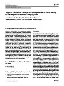
Various ways of incident HPM wave coupling to an electronic system

Part1 Background  IBM Corporation

HPM energy flows into transistors Printed Circuit Board

Transistor

Chip

Part1 Background Because the characteristic length of semiconductor device is relatively smaller than the wavelength of HPM, the energy deposit can be neglected. Unfortunately, PCB wires are efficient antennas which can receive HPM energy. In this thesis, transistors only stimulated by current or voltage sources come from chip pins.

Part2 Semiconductor Physics S. M. Sze, Physics of Semiconductor Devices, 2nd ed. (New York: John Wiley & Sons, 1981). „ „ „

Band structure Fermi-Dirac distribution Classical Boltzmann Transport Equation

Part3 Numerical Methods „ „ „ „ „ „

Governing Equations Finite Volume Method Discretization Boundary Conditions Nonlinear Solvers Linear Solvers

Governing equations of HDM We only present equations for electrons here

G ∂n + ∇ ⋅ ( nv ) = − R ∂t

G * G G ∂ ( m nv ) m nv * GG + ∇ ⋅ (m nvv ) + ∇(nkT ) = −enE − τp ∂t *

G G G G nw − 2 / 3nkTL ∂ ( nw) + ∇ ⋅ (nvw) + ∇ ⋅ (nkTv ) = −env ⋅ E − ∂t τw

ρ ∇ ϕ=− ε 2

If we simplify HDM, just drop energy equation and the first two items of moment equation,that is DDM.

Conservation form The governing equations can be present in conservation form. ∂Q ∂Fi + = S ⋅Q ∂t ∂xi  n   * G m nv   Q=  nw     0 

G nv    * GG  m nvv + nkT   F= G G  nwv + nkTv    ∇ϕ  

S ⋅ Q is the source item

Finite Volume Method Use Gauss’s law, the integration of the partial item over the control volume can be replaced by boundary integration. That is

∂ QdV + v∫ Fi ⋅ ds = ∫ S ⋅ QdV ∫ ∂t

Or the semi-discrete form: dQ Vcell + ∑ Fi ⋅ l = S ⋅ QVcell dt

Q S is the average value of the cell.

Discretization How to get the flux at the boundary of cell is the key problem of FVM. A good HD scheme must satisfy high resolution, nonoscillation and total variation diminishing. In modern CFD world, least-squares reconstruction with limiters, flux upwindsplit and dual-time implicit stepping methods are widely used. Each of them has an uncountable number of papers.

Boundary Conditions „ „ „ „

Ohmic BC Schottky BC Gate Contact of MOS Structure *Current Boundary Condition

Current Boundary Conditions The Newton’s method fails to get convergence at the breakdown region if voltage boundary condition is used. Therefore, current BC must be applied to satisfy the requirement of HPM simulation.

Nonlinear Solvers The key process of semiconductor simulation is how to solve the large scale, nonlinear equations arising from discretization step. A flexible, stable and fast arithmetic must be implemented. „ „ „

Basic Newton Line Search Trust Region

Newton’s Method

f ( x) = 0

J k δ k = − f ( xk ) xk +1 = xk + δ k Fast arithmetic: quadratic convergence But only convergence when x → x* Only used in IV curve tracing or transient simulation.

Line Search J k δ k = − f ( xk ) xk +1 = xk + αδ k The first equation only determine the descent direction. Then the step size alpha is solved by a safeguarded polynomial interpolation of f(x). This arithmetic only holds when Jacobian matrix is exact or nearly exact. GSS tried its best to get exact Jacobian matrix, so line search is the default nonlinear solver for get a initial solution.

Trust Region

Bk = J k + λI This method uses positive definite matrix B instead of J to reduce the step size. A sufficient small step size may satisfy toyler series and get convergent gradually. Early edition of GSS didn’t have exact Jacobian matrix, trust region was applicable. But now, line search method is recommended.

Linear Solvers All the Nonlinear solvers request a fast linear solver. In most of the situation, an approximate linear solver is enough. „ „

„

LU Factorization Method Fixed Iterative Method (GS,SOR,SSOR) Krylov Subspace Method (CG,GMRES,BICG)

Part4 Introductions of GSS „ „ „ „ „ „

Pre-processor Model File Format Command File Syntax Flexible Material Database Build-in Solvers Post-processor

GSS 0.42 „

What is GSS? GSS is a General-purpose Semiconductor Simulator. Besides several libraries, version 0.42 has more than 20000 lines of c++ code.

GSS 0.42 have these features „ Use CGNS as standard input/output file format „ Run time parameters are specified by cmd file „ Unstructured mesh(triangle/rectangle) support „ Adaptive mesh refinement „ Two build-in solvers : DDM and HDM

Software Structure of GSS User Input

Graphic Plot

Mesh

Date

Main Control Unit

Solver 1

Solver 2

Solver n

Physical Model Interface

Si

Ge

GaAs

III-V compound

Pre-Processor GSS support Medici compatible model description language, which can build device model, do mesh division and adaptive mesh refinement easily. Beside that, some auxiliary tools can be used as pre-processor.

SGrid: Another Pre/Post Processor

Interface to Other Software GSS can employ Sgframework or Medici to generate device description file. While a small tool TIFTOOL can convert Medici TIF file to CGNS file, which can be read by GSS.

CGNS, The I/O File Format CGNS: CFD General Notation System „

„

„

„

Supported by NASA and many commotional CFD Corporations. Mesh, boundary condition and solution data are stored in one file. Freeware Adfviewer and Cgnsplot can help for debugging. CGNS is well supported by ICEM CFD10.0, the world’s top pre/post processor.

View CGNS file

Show Mesh

Mesh editor (by ICEM)

Post process (by ICEM)

Command file At present, lex and yacc are used to parse command file. It contains:

„

Various run time parameters Boundary condition Voltage source attached to BC

„

Solver specification

„ „

An example of command file 1

An example of command file 2

An example of command file 3

An example of command file 4

Graphic plot „

„

„

„

GSS requests Xwindow to do graphic plot. Support both 2D mesh displaying and 3D plotting of results. User can choose style, color and change view angle by mouse. In the future, Graphic user’s interface will be built.

Solvers „

The two popular methods in semiconductor simulation—DDM and HDM—are supported both.

„

Use DDM method to get a zero bias solution is very fast and accurate while HDM needs a lot of time to get convergence.

„

HDM is suit for sub-micron device simulation such as MESFET and HEMPT

DDM Level 1 DDM is the basic method for semiconductor simulation.It employs Newton’s iterative method to solve nonlinear equations. With the help of PETSC, the DDM solver is ready to go. Because PETSC support line search and trust region method, GSS can get convergence in most of the situation.

DDM Level 2 The thermal effects are critical when device attacked by HPM. Beyond the basic DDM solver, a lattice temperature corrected DDM solver (L2) is developed, which can simulate the thermal phenomena of devices. Unfortunately, DDM L2 runs 2-10 times slower than original edition.

Example 1 PN diode

Original mesh

Potential distribution of equilibrium

Refined mesh

Example 1 PN diode

IV: backward

IV: forward

Example 1 PN diode

Temperature Distribution of forward bias

Example 1 PN diode

Frequent dependent simulation

Example 1 PN diode

Top left: 1MHz Top right: 100MHz Bottom left: 1GHz

Example 2 BJT circuit

Circuit scheme

Input file

0.701

0.00195

0.700

0.00190

0.699

0.00185

Ib (mA)

Vbe (V)

Result of Transient simulation

0.698

0.00180

0.697

0.00175

0.696

0.00170

0

1

2

3

4

5

0

1

2

time (us)

3

4

5

3

4

5

time (us)

2.72 0.070

2.71 0.068

2.70

Ic (mA)

Vce (V)

0.066

2.69

0.064

2.68 0.062

2.67 0.060

2.66 0

1

2

3

time (us)

4

5

0

1

2

time (us)

Example 3 multi-region NMOS Here, a very complex NMOS transistor is simulated, which shows the multi-region processing capacity of GSS.

Mesh Structure

EQUILIBRIUM Potential

Potential Distribution of Vgs =3V, Vds=3V

Example 3 multi-region NMOS

IV curve of Vgs=3V

HDM „

At present, both explicit and implicit HDM method are ok. The Roe and AUSM schemes are supported.

„

The HDM solver is consisted of two main parts: a Poisson solver and a CFD solver. Optimization of Poisson and CFD solver is a future project.

limitation of HDM I did several tests with some transistors. The Numerical viscosity may cause terrible problems in bipolar transistor. HDM works well only with single carrier transistors such as MESFET and HEMT. As a result, adaptive mesh refinement and second order reconstruction in space are done for anti-viscosity. In the future, higher order Discrete Galerkin method may be introduced into GSS.

HDM example GaAs MESFET

Result of MESFET

Electron density

Potential

IV curvy

HDM example NMOS Simplified NMOS Model. Na is set to zero. Only electron was considered.

Doping :Nd

Result of NMOS under Vds=5V, Vgs=5V

Potential

Future Works „

„ „

Build user-friendly Graphic User’s Interface. support heterojunction device. Support optical mechanism.

*Support of FEM For meeting the challenge of CCD simulation, GSS had introduced a background mesh, which enables using FEM to solve electromagnetic problems.

A PN diode with background mesh

*Run GSS on a Cluster „

„

Since GSS support multi-region mesh, to write a parallel edition of GSS is not so difficult. The nonlinear solver itself is well designed for cluster.

Special Thanks for Your Attention! Presented by Gong Ding