Localization Algorithm in Wireless Sensor Networks with Network ...

S.-H. Hong et al.: Localization Algorithm in Wireless Sensor Networks with Network Mobility

1921

Localization Algorithm in Wireless Sensor Networks with Network Mobility Sung-Hwa Hong, Byoung-Kug Kim, and Doo-Seop Eom Abstract — This paper describes a localization algorithm necessary for building small-sized network's position reporting system using wireless sensor network. In existing sensor networks, much of the localization algorithm is devoted to making position estimations by learning a minimum of 3 position values of anchor node that's aware of absolute position value under the environment where sensor nodes are fixed. The proposed algorithm has an indefinite traveling direction and has shown in performance analysis that it is possible to estimate positions even with a small number of anchors. Also, by using the implemented board, although practicality has been proven with implementation of realistic distance measurement through distance measurement using RSSI(Received Signal Strength Indication) and traveling distance measurement using acceleration sensor 1. Index Terms — Sensor Network, Localization, Network Mobility.

I. INTRODUCTION Recently, in the NEMO(Network Mobility Support), the network system in which we use the wireless sensor networks is developed. However, the applications of the sensor network were unable to be still studied as much as they applied to the mobility. The localization problem is more serious. Presently, PRE (Position Reporting Equipment) is the electrical field visibility equipment of the military by using GPS(Global Positioning System) can know the location of the company. Expensive GPS equipment has decreased accuracy in a building or forest. One solution is to use the technology of wireless sensor networks in the position reporting system. Existing localization schemes usually focus on static sensor networks where the sensor nodes do not move once they are deployed, and sensor nodes that are not in the range of at least three anchor nodes cannot estimate their location. In sensor networks it is often difficult to set up three anchors to cover all sensor nodes. In this paper, we propose simple localization schemes for a small unit position reporting system in wireless sensor networks. The first proposed scheme is a very simple localization system for wireless sensor networks that do not rely on multiple anchors, but it is a directional-antenna-based scheme. The second proposed scheme is applicable to mobile sensor networks which do not have specific ranging hardware and instead require only accelerometers and digital compasses. 1 . Sung-Hwa Hong is with the Dep. of Software Engineering, Dongyang Technical College, Seoul, Korea. (email: shhong,@dongyang.ac.kr) Byoung-Kug Kim and Doo-seop Eom are with the Dep. of Electronics and Computer Engineering, Korea University, Seoul, Korea. (email: {dearbk, eomds}@final.korea.ac.kr)

Contributed Paper Manuscript received September 20, 2009

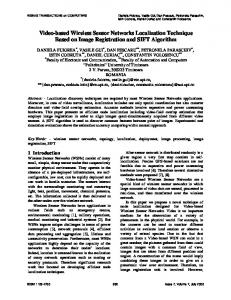
Section II discusses related works. Section III describes our suggested algorithms, and section IV shows the simulation results of our proposed algorithms. Finally, we offer concluding remarks in section V. II. RELATED WORKS He et al. [1] presents a range-free localization algorithm in which RSS values are obtained from signals of the anchors by calculating the distances between unknown nodes and anchors. Alippi and Vanini [2] present a multi-hop localization technique for wireless sensor networks based on RSSI(received signal strength indication), using the collected RSSI values at different power levels of nodes to build the ranging model in a centralized minimum least square algorithm to estimate the location of nodes. A scheme tolerant to anisotropic network scenarios [3] uses multidimensional scaling (MDS) to calculate the relative positions of the unknown nodes; the absolute positions are determined using coordinate alignment techniques. With the assistance of a moving target, a deterministic constraint-based localization approach is proposed in [4] which uses bounding rectangles and negative information. In [5], a node localizes itself at the centroid of the overlapped transmission coverage regions of the beacon nodes. In [6] a set of connectivity constraints is built and used to discover the location by convex optimization. In [7], an area-based, range-free localization scheme is described in which the position uncertainty of an unknown is reduced by using the triangles formed by all of the beacons that can be heard by that unknown. III. PROPOSED ALGORITHM A. Localization using the directional antenna The first method is a localization technique using directional antenna. Here it is assumed that the anchor node is capable of transmitting each sector's azimuth with one's absolute position information and sector antenna using GPS module, sector antenna, and digital compass. The sector antenna posses directivity so that the transmission is possible only within certain angle ranges. For example, in 2-sector antenna each sector has 180 degrees of directivity, while for a 4-sector antenna, the transmission is possible within a 90degree range for each sector. Using these sector antennas, absolute position information is loaded in the beacon for transmission, and the received sensor nodes can localize their respective positions using trigonometric function as in Fig. 1.

0098 3063/09/$20.00 © 2009 IEEE

1922

IEEE Transactions on Consumer Electronics, Vol. 55, No. 4, NOVEMBER 2009

Again, after the anchor node rotates counter-clockwise by θW/M of beam width, the central angle of each sector is as follows, where M is an integer larger than 1. 1st sector : π/N − 2π/NM = 2π/N(1/2−1/M) + θ 2nd sector : 3π/N − 2π/NM = 2π/N(3/2−1/M) + θ Nth sector : 2π/N(N−1/M) + θ Fig. 1 Localization using trigonometric function.

When an anchor node's position is (Xa,Ya), the sensor node's position (X,Y) is obtained as in the following formula. X = Xa + d·cosθ Y = Ya + d·sinθ Here, the sector antenna's azimuth θ can be found with a digital compass, and the digital compass's sensor provides angles between 0 and 359°, with a resolution of 0.1° and an absolute precision of 3°. The value is 0 if the anchor node's sector antenna is facing north and 90 when facing west. The distance, d, between the sensor node and anchor node is found using RSSI (received signal strength indication). It is assumed that the anchor node loads several sector antennas in line with sector's beam width, is capable of transmitting the azimuth in each sector, and covers all directions, as shown in Fig. 2(a)

(a) (b) Fig. 2 (a) The sector antenna’s azimuth, (b) The real sector antenna’s azimuth .

If the antenna's beam width is expressed as θw, the number of antennas is given by the following expression: N =

2π θϖ

The greater the number of sector antennas, the smaller the beam width gets, thus raising accuracy but making it harder to actually build the system. Although in reality the emission pattern of sector antennas has an irregular pattern as in Figure 2(b), this paper will assume that there is a constant beam width of θw. When the anchor node has N sectors as in Figure 2(a), and each sector's beam width is θW = 2π/N and the digital compass's azimuth is θ, the central angle is π/N +θ for the first sector, 3π/N +θ for the second 2 sector, and 2π-π/N +θ for the Nth sector. Using each sector's central angle and the distance, d, provided by RSSI, the sensor node estimates its position (Xi,Yi) and stores it.

After rotating by θW/M, the sensor node's position (Xi,Yi) is estimated and stored in the same way. Here the sensor node repeats M times in estimating and saving the position, after which point an average value is calculated as below in order to determine the final position (X, Y). X =

M

∑

i=1

(

Xi ) M

Y =

M

∑

(

i=1

Yi ) M

For example, if that the digital compass's azimuth θ is 0 and it is made up of 6 sectors as in Figure 3, each sector's beam width becomes 2π/6, or 60o. If the beam width's central angle is transmitted, the first sector is π/6, the second sector is π/2, and the sixth sector is 11π/6. When there are nodes A and B located the same distance from the anchor node and within the first sector reception radius, and when the position calculation is made with the proposed algorithm, π/6 is applied to both nodes in being expressed as a single point in the first sector's center line.

Fig. 3 A, B node location calculation in the 1st sector.

the anchor node's position is (0,0) and the distance d between A and B is 30 m, the positions of nodes A and B are estimated as follows. X = 0 + 30*cos(π/6) = 25.98 Y = 0 + 30*sin(π/6) = 15 The positions of A and B are approximately 26 and 15. In the next stage, when the anchor node has rotated counterclockwise by π/6, as in Figure 4, and when the positions of both nodes are calculated as above, the A node is at (30, 0) and the B node is at (15, 26). Each node stores the position information of their own in the memory and calculates the average of each respective position value in determining the final position of their own. Therefore, the position of the A node is (28, 7.5) and that of the B node is (20.5, 20.5). Here, the accuracy of the localization increases when using antenna with a smaller sector beam width loaded in anchor

S.-H. Hong et al.: Localization Algorithm in Wireless Sensor Networks with Network Mobility

node, and when the average of M position values is calculated by reducing the rotation angle by 1/M rate of sector beam width, results closer to actual position will be derived.

Fig. 4 The beacon transmission after the anchor node has rotated by π/6.

1923

B. Localization using the acceleration sensor The second localization algorithm is a localization technique that uses dead reckoning. Each node is loaded with an omni-directional antenna, and it is assumed that one's traveling distance and direction can be determined with an accelerometer and digital compass. In an environment where the nodes move as illustrated in Figure 7, the sensor node receives an anchor node's position information when that anchor is within a certain communication radius, and it modifies the received anchor node's position information by taking into account the distance traveled and the direction, which are stored in memory. Whenever there is information from at least 3 sensor nodes, the position is determined by performing localization through trilateration.

As illustrated in Fig. 5, the localization technique using directional antennas can be summarized.

Fig. 7 Localization of the sensor S1 met 3 anchor.

Fig. 5 The flowchart of a localization using the directional antenna.

As most existing localization algorithms require receiving at least 3 beacons in order for the sensors to estimate position, if the anchors and sensor nodes are moving, the previous beacon's information becomes the reason for a large error upon receiving the next beacon. However, as the algorithm described here calculates position immediately when the sensor node receives the beacon sent by anchor node and the position of sensor nodes are estimated in a single beacon interval, it is adequate for a mobile environment's localization algorithm in Fig. 6.

Fig. 6 A sensor node position estimation in the beacon signal interval.

Here, the distance d between the anchor and sensor is obtained using RSSI. In an environment such as military operations where a certain distance is maintained between nodes and troops move in the same direction, the probability that a sensor node will detect at least 3 anchor nodes with absolute coordinates within 1 hub range is remote. Even if the sensor node has estimated its position with information from at least 3 beacons, the angle θ error from the accelerometer and digital compass will increase steadily as time passes, enlarging the error tolerance and making the estimated position unreliable. To complement this information, the node S1 has beacon information for anchors A1 and A 2 in its memory as in Figure 8, and it is capable of estimating its position as it receives information from its neighboring node S2 about anchor A 3. Of course, node S 2 is also capable of estimating its position by receiving beacon information about anchors A 1 and A 2 from node S 1. That is, as an anchor's absolute position and distance value provided by RSSI are shared among nodes, each node increases its probability of having information from enough anchors to estimate its position.

1924

IEEE Transactions on Consumer Electronics, Vol. 55, No. 4, NOVEMBER 2009

and the coordinate matrix of the node with unknown position x can be obtained as follows using least-squares:

xˆ = (AT A)-1 ATb

Fig. 8 Localization of the sensor S1 met 3 anchor.

When at least 3 beacons are registered in node S1's memory with information about their absolute coordinates and distance, the node’s position is estimated through trilateration. Trilateration is the key technique in distance-based localization, and as it requires solving only a number of linear equations equal to the number of considered reference nodes, it is a very simply localization technique. Thus the calculation speed is fast and has a low system burden. Let the coordinate matrix of the anchor node be Ri = (xi, yi)T, i = 1, 2, ‚‚‚, m, where m is the number of anchor nodes, and let the coordinate matrix of the node with unknown position be x = (x, y)T. The values in the coordinate matrix of the node with unknown position x are given by the solutions to following equations. ( x 1− x )2 + ( y1 − y )2 = d 1

2

Dead reckoning technology is used as a supplementary position tracking navigation technology in those places where GPS doesn't operate; in these cases a node’s position can be estimated by determining the distance and direction the node has traveled with an acceleration sensor and digital compass. Using an acceleration sensor, the node's traveling distance can be calculated as follows. The acceleration a is the change of speed per unit time, and the speed s is the change of distance per unit time. Therefore, the change of speed is calculated by multiplying the acceleration by the time t, and speed s can be calculated by adding the change in speed to the initial speed s0 as follows. s = s0 + a·t By knowing the speed, it is possible to calculate the distance traveled during a unit of time. The distance traveled l is calculated by multiplying time by speed as follows.

l = s·t The traveling direction θ is obtained through the digital compass.

# (x

m

− x)

2

+ ( ym − y )2 = d

2 m

By subtracting each of the first m-1 equations from the final equation, one can obtain the following m-1 equations 2 x ( x 1 − x m ) + 2 y ( y1 − y m ) = d m2 − d 12 + x 12 − x m2 + y12 − y m2 #

2 x( x m−1− xm ) + 2 y( ym−1 − ym ) = d m2 − d m2 −1 + xm2 −1 − xm2 + ym2 −1 − ym2 Fig. 9 Node repositioning using trigonometric function.

which can be expressed in matrix form as follows:

Ax = b

When the A1 node's initial position is A1(x1,y1), as in Figure 9, the position A1’(x1’,y1’) after time t can be calculated as follows.

Here, A and b are given by ⎡ x1 − x m A = ⎢⎢ # ⎢⎢ x m − 1 − x m

x1’ = x1 + l·sinθ

y1 − y m ⎤ ⎥ # ⎥ y m − 1 − y m ⎥⎥

⎡ ( d m2 − d 12 + x 12 − x m2 + y 12 − y m2 ) / 2 ⎢ b= ⎢ # ⎢ ( d m2 − d m2 − 1 + x m2 − 1 − x m2 + y m2 − 1 − y m2 ) / ⎢

y1’ = y1 + l·cosθ ⎤ ⎥ ⎥ 2 ⎥⎥

The position of the node obtained in this way is stored in the sensor node's memory, and when the sensor node moves, the positions of the beacon nodes stored in memory are recalculated as above.

S.-H. Hong et al.: Localization Algorithm in Wireless Sensor Networks with Network Mobility

1925

- Sector antenna's beam width: As the angle received by sensor node receives each sector's central angle, it is assumed that there is no error for the sector antenna's beam width θW. - Embedded sensor module (acceleration sensor, digital compass, GPS) error: It is assumed that there is no error from the acceleration-measuring sensor, the digital orientation instrument for measuring orientation and angle, and the GPS module. B. Simulation scenario After randomly distributing anchor nodes and sensor nodes in a perfect square sensor field of dimensions 200 × 200 m2 as shown in Figure 11, the simulation assumes movement in different directions within the maximum speed that a human can move. Using the parameter shown in Table 1, 30 tests were performed and an average value was obtained. TABLE I THE SIMULATION PARAMETERS

Fig. 10 The flowchart of a localization using the acceleration sensor.

The localization technique that uses an acceleration sensor and digital compass can be summarized as shown in Fig. 10.

Anchor radio range

IV. PERFORMANCE ANALYSIS This section describes a test of the performance of the algorithm proposed in Applicable Localization Algorithm with NEMO, and it analyzes the effects of measurement error. In the simulation, the following testing conditions are assumed. A. Simulation measurement standards and error factor The following measurement standards are used for simulation analysis. - Average position error: Average distance between expected position (Xei, Yei) and actual position (Xi, Yi) obtained through calculation of all sensor nodes. Average location error =

∑

Value(s)

Parameter

Directional antenna : 100m Omni-antenna : 50m

Node radio range(R) Number of anchor Number of node Number of direct6ional antenna Max. moving speed

50m 1, 2, 3, 4, 5 10, 20, 30, 40, 50 2, 3, 4, 5, 6, 7, 8, 9, 10 1.5m/s, 3m/s, 5m/s

RSSI error

0.05

( X ei − X i ) 2 + (Y ei − Y i ) 2 Number of sensor

Assumptions for likely error factors are as follows. - RSSI value error: RSSI value, the measurement of distance value between the anchor and sensor node, is theoretically inversely proportional to the square of the distance, thus decreasing the signal's strength. However, error occurs during the actual measurement because of environmental factors. As RSSI has an error value of about 0.05 under normal circumstances, it was applied the same way in simulation. - Node's speed: The distance value traveled during the position estimation time is the cause of the error. That is, the faster the speed, the higher the error value. Here, the speed of testing nodes is assumed to be the speed of human travel (1.5 m/s when walking, 3m/s, 5m/s when running).

Fig. 11 The simulation topology.

C. Performance analysis for the localization using Directional antenna Recently, directional antennas have been widely applied in sensor networks in terms for the purposes of security and energy efficiency. The simulation here assumed that a multidirectional antenna, that is, a sector antenna, was used.

1926

Fig. 12 Position error according to sector and number of rotations.

Figure 12 shows the average localization error as a function of the number of sectors in an antenna. The angle covered by a sector gets smaller as the antenna's number of sectors increases, thus reducing localization error, as can be seen in the figure. However, although the sector antenna's performance improves as the number of sectors increases, more sectors lead to greater complexity in the antenna and more problems in manufacturing the system. Sending each beacon 2, 3, or 4 times by rotating 1, 2, or 3 times for a beam width of 1/2, 1/3, or 1/4 produced better results than estimating the position with a single beacon without rotation. However, even if the number of beacons increased by 2, 3, or 4 times, there wasn't much gap in position error, while increasing the number of beacons increased the delay time and thus was inefficient. The result was that the case of 6 directional antennas and 2 beacons showed the best results. Therefore, in the next simulation, we continue the method of sending the beacon twice with 6 sector antennas.

IEEE Transactions on Consumer Electronics, Vol. 55, No. 4, NOVEMBER 2009

Fig. 14 The average position error at various speeds as a function of the number of nodes.

Figure 14 shows average position error as various speeds as a function of the number of nodes; it can be seen that there is not much change in the position error even if the node concentration rises sharply. The explanation for this is that because the sensor node within an anchor node's communication radius estimates position only with the anchor's beacon information, the position estimate is unrelated to the concentration of sensor nodes. D. Performance analysis for the localization using the acceleration sensor Just like the algorithm that uses a directional antenna, the algorithm that uses an acceleration sensor also assumes movement in a certain direction within a certain range of speeds with randomly distributed nodes in a sensor field of dimensions 200 × 200 m2. The simulation results indicate that, as shown in Figures 15 and 16, position error increases as the speed of the nodes increases. However, compared with the previously described algorithm which used directional antennas, in this case the amount of change in the position error was small. This is because algorithms that use acceleration sensors are likely to receive anchor information as the speed of the nodes increases. In Figure 15 we can see that there is not much change in position error with a rise in the number of anchors. However, as Figure 16 shows, position error decreases gradually as the number of nodes increases.

Fig. 13 The average position error for various speeds as a function of the number of anchors.

Figure 13 shows the average position for various speeds as a function of the number of anchors. As can be seen, the greater the number of anchors, the smaller the average error. In addition, the error increases as the traveling speed increases because the gap between the calculated position at the point the sensor node receives the beacon from the anchor and the position after traveling gets larger as the speed increases. Because the algorithm that uses sector antenna estimates a sensor node's position with 1 to 2 beacons from the anchor, shortening the beacon gap could reduce errors due to speed.

Fig. 15 Position error at various speeds as a function of the number of anchors.

S.-H. Hong et al.: Localization Algorithm in Wireless Sensor Networks with Network Mobility

1927

F. The implementation of this algorithm

(a) A front of the main

(b) A back of the main

Fig. 16 Position error at various speeds as a function of the number of nodes.

E. Comparison with existing algorithm To compare the proposed algorithm was compared with the existing localization algorithms, 10 sensor nodes and 3 anchor nodes were randomly distributed in a sensor field of dimension 500 × 500 m2, with all of them traveling at a speed of 3m/s. The results of the comparison are shown in Fig. 17, which graphs the position error as a function of the passage of time. As can be seen, the localization errors in the proposed algorithm I and in the MCL [8] algorithm gradually decreases with time.

(c) The interface

(d) The acceleration sensor

Fig. 18 The implemented module and the acceleration sensor.

For the actual implementation of the proposed localization technique, we used the sensor node manufactured in the laboratory to test the distance measurement between nodes using RSSI and the node's traveling distance measurement using the acceleration sensor. V. C ONCLUSION

Fig. 17 Comparison with existing algorithm.

As MCL becomes more likely to meet an anchor as the nodes travel faster, the initial error is very large because at least 50 positions should be sampled even if the error decreases. As DV-distance algorithm calculates one's position using information from anchors 2–3 hubs away, a large amount of error appears in environments where nodes travel when compared to other algorithms. As can be seen in Figure 17, the proposed algorithms Ⅰ and Ⅱ show the least amount of position error as a function of time at the speed at which humans can move (3m/s). Although algorithms that use directional antennas have better results among the various proposed algorithm, the algorithms that use acceleration sensors and digital compasses are more efficient in actual realization aspect.

The existing sensor network, the majority of localization algorithms are capable of estimating position by knowing at least 3 position values for anchor nodes aware of absolute position values in an environment where the sensor nodes are fixed. However, this paper has proposed localization algorithms that estimate the position of nodes that continuously move with sensor nodes attached and traveling nodes by gate nodes attached with anchor nodes. As the existing algorithm [9] assumes that the antenna emission pattern is completely round and moves in a certain direction, and [8] estimates with probability calculation under the assumption that the traveling direction and speed are fixed, the error and delay time for localization are large. However, the proposed algorithm has an indefinite traveling direction, and it has shown in performance analysis that position estimation is possible even with a small number of anchors. It was confirmed that the 2 proposed algorithms are more efficient than the existing algorithms. Also, although we have shown that it is practical to implement realistic distance measurements through distance measurements using RSSI and traveling distance measurements using an acceleration sensor, further work is needed in a number of areas. Further research needs to be done into such hardware as sector antennas adequate for transmission and reception of sensor nodes, and additional energy-efficient algorithms are needed in order to make additional improvements in the system.

1928

IEEE Transactions on Consumer Electronics, Vol. 55, No. 4, NOVEMBER 2009

REFERENCES [1] [2]

[3] [4]

[5] [6] [7] [8] [9]

HE T., HUANG C., BLUM B., STANKOVIC J., ABDELZAHER T.: ‘Range-free localization schemes in large scale sensor networks’. Proc. MobiCom’03, ACM Press, San Diego, 2003, pp. 81–95 ALIPPI C., VANINI G.: ‘A RSSI-based and calibrated centralized localization technique for wireless sensor networks’. Proc. 4th Annual IEEE Int. Conf. Pervasive Computing and Communications Workshops (PERCOMW’06), Pisa, Italy, 2006, pp. 301–305 X. Ji and H. Zha, “Sensor Positioning in Wireless Ad-hoc Sensor Networks Using Multidimensional Scaling,” in Proc. of IEEE INFOCOM 2004, Mar. 2004, pp. 2652–2661. A. Galstyan, B. Krishnamachari, K. Lerman1, and S. Pattem, “Distributed Online Localization in Sensor Networks Using a Moving Target,” in the third international symposium on information processing in sensor networks, 2004, pp. 61–70. N. Bulusu, J. Heidemann, and D. Estrin, “GPSless low cost outdoor localization for very small devices,” IEEE Personal Communications Magazine, vol. 7, pp. 28–34, Oct. 2000. L. Doherty, K. S. J. Pister, and L. E. Ghaoui, “Convex position estimation in wireless sensor networks,” in Proc. IEEE INFOCOM 2001, vol. 3, Anchorage AK, Apr. 2001, pp. 1655– 1663. T. He, C. Huang, B. M. Blum, J. A. Stankovic, and T. Abdelzaher, “Range-Free Localization Schemes for Large Scale Sensor Networks,” in Proc. of ACM MobiCom 2003, 2003, pp. 81–95. Lingxuan Hu, David Evans, “Localization for Mobile Sensor Networks”, MobiCom 2004, Sept. 26. K. F. Ssu, C. H. Ou, and H. C. Jiau, “Localization with Mobile Anchor Points in Wireless Sensor Networks,” IEEE Transactions on Vehicular Technology, vol. 54, no. 3, pp. 1187–1197, May 2005.

Sung-Hwa Hong received his B.S.degree in Computer Science from Seoul, Korea University, 1996 and his M.S. degrees in Information and Communication Engineering from Hankuk Aviation University, in 2002. In 2008, he received his Ph.D. degree in Electronics and Computer Engineering from Korea University, Seoul, Korea. From March 2008, he has been an instructor in the Department of Software Engineering at Dongyang Technical College. His research interests include the Home Network, WLANs, ad-hoc networks. Byoung-Kug Kim received his B.S. degree in Computer Engineering from Won Kwang University, Iksan, Korea, 2002, and his M.S. degree in Electronics and Computer Engineering from Korea University, Seoul, Korea, 2004. Since 2004, he has been in the Ph.D program in Electronics and Computer Engineering at Korea University, Seoul, Korea. His research interests include Bluetooth, embedded-system, ad-hoc and sensor networking, and ubiquitous computing. Doo-Seop Eom received his B.S. and M.S. degrees in Electronics Engineering from Korea University, Seoul, Korea in 1987 and 989, respectively. In 999, he received his Ph.D. degree in Information and Computer Sciences from Osaka University, Osaka, Japan. He joined the Communication System Division, Electronics and Telecommunications Research Institute (ETRI), Korea, in 1989. From September 2000, he has been an associate professor in the Department of Electronic Engineering at Korea University. His research interests include communication network design, Bluetooth, ubiquitous networking and Internet QoS.