Hindawi Shock and Vibration Volume 2017, Article ID 6106103, 9 pages https://doi.org/10.1155/2017/6106103
Research Article A Spectrum Detection Approach for Bearing Fault Signal Based on Spectral Kurtosis Yunfeng Li, Liqin Wang, and Jian Guan School of Mechanical Engineering, Harbin Institute of Technology, Harbin, China Correspondence should be addressed to Liqin Wang;
[email protected] Received 2 August 2016; Revised 9 November 2016; Accepted 4 December 2016; Published 19 February 2017 Academic Editor: Angelo M. Tusset Copyright © 2017 Yunfeng Li et al. This is an open access article distributed under the Creative Commons Attribution License, which permits unrestricted use, distribution, and reproduction in any medium, provided the original work is properly cited. According to the similarity between Morlet wavelet and fault signal and the sensitive characteristics of spectral kurtosis for the impact signal, a new wavelet spectrum detection approach based on spectral kurtosis for bearing fault signal is proposed. This method decreased the band-pass filter range and reduced the wavelet window width significantly. As a consequence, the bearing fault signal was detected adaptively, and time-frequency characteristics of the fault signal can be extracted accurately. The validity of this method was verified by the identifications of simulated shock signal and test bearing fault signal. The method provides a new understanding of wavelet spectrum detection based on spectral kurtosis for rolling element bearing fault signal.
1. Introduction The rolling element bearing is one of the most important parts in aircraft engines. Many bearing incidents in aircraft engines have indicated that the initial damage of bearing occurred on the surface and subsurface. This initial damage appears as the peeling and develops into spalls eventually [1]. During the performance and reliability testing, the vibration signal can reveal the failure state in time and frequency domain promptly. In order to obtain the fault characteristic parameters of the rolling bearing, a variety of signal processing methods are applied to process the rolling bearing vibration signal. Since wavelet transform has the property of time-frequency localization, it is utilized to detect the signal transients from the raw signal extensively [2–6]. The wavelet transform provides an analysis method both in time domain and in frequency domain, which becomes an important method in the nonstationary signal analysis. It is well known that the similarity exists between Morlet wavelet and the impact response of the attenuation components, and the Morlet wavelet is Gaussian in the frequency domain. In addition to the above factors, the time-frequency structure of the Morlet wavelet is optimal match with the typical transients. Therefore, the Morlet wavelet is more suitable for the extraction of rotating machinery fault signal and the rolling bearing fault diagnosis.
The purpose of wavelet transform is to select the proper frequency band of the correct faulty information and the best filter. Therefore, it is necessary and urgent to select the reasonable resonance frequency band for the demodulation technology. At the same time, an index unaffected by experimental conditions is needed to measure the transform result. Kurtosis is a normalized time domain statistics parameter, which is sensitive to the instantaneous signal. Thus, the spectral kurtosis (SK) is an effective tool to get the fault signals of rolling bearing and the reasonable bandwidth [7, 8]. SK is used to analyze the Gaussian components of the signal and locate these components in the frequency domain. It can be seen as a measurement of the energy distribution at each frequency. The peeling of the faulty bearing produces a nongauss distribution signal, which can be described by the time averaging statistic. The final purpose of SK is to detect the fault signal characteristics in the filtering results [9–11]. The concept of SK was proposed by Dwyer firstly [12]. Then, it was successfully applied to the rolling bearing resonance peak and resonance band selection by Antoni and Randall [13]. Fast Kurtogram based on band-pass filter and short-time Fourier transform (STFT) has made SK a practical tool for the fault diagnosis [14]. Nevertheless, in order to obtain a maximum value of the spectral kurtosis, the STFT window must be shorter than the spacing between the pulses and longer than the individual pulses. The maximum spectral
2
Shock and Vibration
kurtosis value corresponding to the band is not always the optimal band by the above method. In order to solve these problems, various kinds of improved algorithms based on spectral kurtosis and other signal processing technologies were presented, such as searching all the possible resonance frequency bands adaptively by shifting and expanding predetermined Morlet wavelet [15]. In this paper, the Morlet wavelet and SK are combined. The spline curve function is utilized to obtain the optimal wavelet filter range, and different wavelet clusters are designed to detect the impact frequency. Firstly, a group of Morlet wavelet cluster with different quality factor 𝑄 is designed and the spectral kurtosis of the filtered signal is calculated, respectively. Then, the trend of spectral kurtosis is drawn by the spline curve based on a limited number of points. The signal detection range and filter bandwidth are gradually reduced. As a consequence, the accuracy of fault diagnosis is improved by the optimized filter.
2. Adaptive Spectral Kurtosis Filtering Based on Morlet Wavelet 2.1. Morlet Wavelet. The complex Morlet wavelet is the product of a complex exponential function multiplied by a Gaussian function. The expression of Morlet wavelet is Morl (𝑡) =
𝜎 −𝜎2 𝑡2 𝑖2𝜋𝑓0 𝑡 𝑒 𝑒 . √𝜋
(1)
Meanwhile, the shape of Gaussian window in the frequency domain can be derived as [16] 2
2
2
Morl (𝑓) = Morl∗ (𝑓) = 𝑒−(𝜋 /𝜎 )(𝑓−𝑓0 ) ,
(2)
where Morl(𝑓) is the fast Fourier transformation of Morl(𝑡). Since Morl(𝑓) is real, Morl(𝑓) = Morl∗ (𝑓), and the superscript ∗ denotes the complex conjugate. 𝑓0 is the center frequency of the wave and 𝜎 is waveform parameter that determines its width. For Morlet wavelet, the center frequency 𝑓0 , and shape factor 𝜎 affect the shape and location simultaneously. By (1), the corresponding wave shape of Morlet wavelet is shown in Figure 1. In Figure 1, Morl1 is the wave of the Gaussian function, and Morl2 is the complex exponential wave function. They are expressed as −𝑡2 𝜎2
Morl1 = 𝑒
,
Morl2 = 𝑒𝑖2𝜋𝑓0 𝑡 .
𝑡1 = 𝑡2 =
𝜎
t
t2
t1
Morl Morl1 Re(Morl2)
Figure 1: Structure of Morlet wavelet.
where 𝑚 is the value of Morlet wave endpoint and it is infinitesimal (as shown in Figure 1). It is necessary to ensure that the Morlet wavelet is fluctuant enough and compactly supported. For Morl1 and Morl2, the period ratio 𝑇1 /𝑇2 is 𝑇1 2𝑡1 𝑄𝜋√ln 𝑚−1 = = = 𝑘, 𝑇2 4𝑡2 arccos (𝑚)
(3)
𝑘 arccos (𝑚) 𝑘1 arccos (𝑚) ≤𝑄≤ 2 . −1 √ 𝜋 ln 𝑚 𝜋√ln 𝑚−1
arccos (𝑚) , 2𝜋𝑓0
(6)
The quality coefficient 𝑄 is proportional to the fluctuation of the Morlet wavelet. The larger the quality coefficient 𝑄 is, the smaller the volatility of the Morlet wavelet is and vice versa. Therefore, when 0.5 ≤ 𝑘 ≤ 2 and 𝑚 = 0.00001, the value range of 𝑄 is 0.0217 ≤ 𝑄 ≤ 0.0869. The corresponding family of wavelets consists of a series of son wavelets, which are generated by dilation and translation from the mother wavelet shown as follows: 𝑡−𝑏 1 Morl ( ), √𝑎 𝑎
(7)
where 𝑎 is the scale factor and 𝑏 is wavelet displacement factor (the constant 1/√𝑎 is used for energy normalization). The wavelet transform coefficient is defined by the following equation: WT(𝑎,𝑏) = ∫
+∞
−∞
,
(5)
where 𝑄 is the quality factor, 𝑄 = 𝑓0 /𝜎. When 𝑘1 ≤ 𝑘 ≤ 𝑘2 , Morlet wavelet at most includes 𝑘2 Morl2 and at least 𝑘1 Morl2. If (5) is introduced into 𝑘1 ≤ 𝑘 ≤ 𝑘2 , the expression of the quality coefficient 𝑄 can be obtained as follows:
Morl𝑎,𝑏 (𝑡) =
According to the Euler formula, Morl2 can be expressed as Morl2 = cos(2𝜋𝑓0 𝑡) + 𝑖 sin(2𝜋𝑓0 𝑡), where Re(Morl2) = cos(2𝜋𝑓0 𝑡). If 𝑡1 is half a cycle of Morl1 and 𝑡2 is a quarter period of Re(Morl2), 𝑡1 and 𝑡2 can be deduced as √ln 𝑚−1
m
𝑥 (𝑡) ⋅ Morl∗𝑎,𝑏 (𝑡) ⋅ 𝑑𝑡
(8)
= ⟨𝑥 (𝑡) , Morl𝑎,𝑏 (𝑡)⟩ , (4)
where Morl∗𝑎,𝑏 (𝑡) is the conjugate complex numbers of Morl𝑎,𝑏 (𝑡) and ⟨⋅⟩ represents solving convolution.
Shock and Vibration
3
2.2. Spline Curve Interpolation. Since the SK values are not continuous, the spline curve is used to obtain the variation trend of SK on the basis of discrete points. It can provide the basis for optimizing the analysis range. The function of spline curve interpolation is an approximation of piecewise three polynomials, but it is continuous. Its first- and second-order derivatives are both continuous. The value of 𝑥𝑗 is 𝑦𝑗 = 𝑓(𝑥𝑗 ) (𝑗 = 0, 1, . . . , 𝑛), spline curve interpolation function is 𝑆(𝑥), and its first-order derivative 𝑆 (𝑥𝑗 ) = 𝑚𝑗 . 𝑆(𝑥) can be expressed as 𝑛
𝑆 (𝑥) = ∑ [𝑦𝑗 𝛼𝑗 (𝑥) + 𝑚𝑗 𝛽𝑗 (𝑥)] , 𝑗=0
(9)
where 𝛼𝑗 (𝑥) and 𝛽𝑗 (𝑥) are the interpolation function, expressed by 𝛼𝑗 (𝑥) 𝑥 − 𝑥𝑗 𝑥 − 𝑥𝑗−1 2 { { ) (1 + 2 ) 𝑥𝑗−1 ≤ 𝑥 ≤ 𝑥𝑗 (𝑗 ≠ 0) ( { { 𝑥𝑗 − 𝑥𝑗−1 𝑥𝑗−1 − 𝑥𝑗 { { { { 2 ={ 𝑥−𝑥 𝑥 − 𝑥𝑗 𝑗+1 { { ) (1 + 2 ) 𝑥𝑗 ≤ 𝑥 ≤ 𝑥𝑗+1 (𝑗 ≠ 𝑛) ( { { { 𝑥 − 𝑥 𝑥 { 𝑗 𝑗+1 𝑗+1 − 𝑥𝑗 { Others, (10) {0 𝑥 − 𝑥𝑗−1 2 { { ) (𝑥 − 𝑥𝑗 ) 𝑥𝑗−1 ≤ 𝑥 ≤ 𝑥𝑗 (𝑗 ≠ 0) ( { { 𝑥 − 𝑥𝑗−1 { { { 𝑗 { 2 𝛽𝑗 (𝑥) = { 𝑥 − 𝑥 𝑗+1 { { ) (𝑥 − 𝑥𝑗 ) 𝑥𝑗 ≤ 𝑥 ≤ 𝑥𝑗+1 (𝑗 ≠ 𝑛) ( { { { { 𝑥𝑗 − 𝑥𝑗+1 { Others. {0
2.3. Transient Signal Detection Based on SK. The nonstationary signal is normally expressed by Wold-Cram´er decomposition; that is, +∞
−∞
𝑒𝑗2𝜋𝑓𝑡 𝐻 (𝑡, 𝑓) 𝑑𝑋 (𝑓) ,
(11)
where the time-varying transfer function 𝐻(𝑡, 𝑓) can be interpreted as the complex envelope or complex demodulate of process 𝑌(𝑡) at frequency 𝑓. The signal characteristics information in 𝐻(𝑡, 𝑓) can be described by the spectral moments, the expression of which is 𝑆2𝑛𝑌 (𝑓) ≜ 𝐸 {𝑆2𝑛𝑌 (𝑡, 𝑓)} =
2𝑛 𝐸 {𝐻 (𝑡, 𝑓) 𝑑𝑋 (𝑓) } 𝑑𝑓
(12)
2𝑛 = 𝐸 {𝐻 (𝑡, 𝑓) } ⋅ 𝑆2𝑛𝑥 .
(13)
(14)
The greater the degree of signal deviation from Gaussianity is, the greater its fourth-order spectral accumulation is. Therefore, the energy normalized fourth-order spectral accumulation can be used to measure the peak of the signal process probability density at the frequency 𝑓, that is, spectral kurtosis. The wavelet coefficients can be obtained by calculating the signal convolution by each row of the filter. The higher value of the wavelet coefficient is, the more similar the wavelet function with the signal waveform will be. The values of the wavelet coefficients are equal to the square of energy. SK is used to measure the energy spectrum. Therefore, SK achieves the maximum value when the waveforms are most similar [16]. Equation (15) gives the value of spectral kurtosis for each filter [18]: kurtosis (𝑦) ≜
𝐶4𝑌 (𝑓) 𝑆4𝑌 (𝑓) = 2 −2 2 (𝑓) 𝑆2𝑌 𝑆2𝑌 (𝑓) mean (𝐻4 (𝑡, 𝑓)) 2
(mean (𝐻2 (𝑡, 𝑓)))
(15)
− 2.
2.4. Construction of Wavelet Clusters. Adaptive wavelet method uses spectral kurtosis as the evaluation index of Morlet wavelet filtered results. This method can optimize the latter filter parameters according to the calculation results in the previous step. Each step can improve the calculation accuracy and reduce the searching scope effectively. Compared with other bearing fault diagnosis method based on kurtosis, the accuracy of fault frequency identification and the detection bandwidth are both optimized. During the construction of octave filter with complex translation Morlet wavelet, the number of filters that cover the entire analysis band is 𝑀 = 𝐾 × 𝑁, where 𝐾 is the number of the filters in each octave and 𝑁 is the number of the octaves [19]. The central frequency of the filter is expressed as 𝑓𝑚𝑘 =
𝑓max − 𝑓min 𝑛 (21/𝐾 )
(𝑛 = 1, 2, . . . , 𝑀) ,
(16)
where [𝑓min , 𝑓max ] is the frequency band range of the bearing characteristic frequencies in the operating mode. Bandwidth of each filter is expressed by 𝜎𝑛𝐾 = 𝑓𝑛𝐾 ⋅
Under the conditions of ergodicity and stationarity of 𝐻(𝑡, 𝑓), it is easy to prove that 𝑆2𝑛𝑌 (𝑓) = ⟨𝑆2𝑛𝑌 (𝑡, 𝑓)⟩𝑡 .
2 (𝑓) . 𝐶4𝑌 (𝑓) = 𝑆4𝑌 (𝑓) − 2𝑆2𝑌
=
Under the condition of corresponding boundary, the function 𝑆(𝑥) can be calculated when the equations of 𝑚𝑗 (𝑗 = 0, 1, . . . , 𝑛) were obtained [17].
𝑌 (𝑡) = ∫
The significant property of nonstationary processes is non-Gaussian. For a non-Gaussian process, spectrum accumulation that is greater than or equal to the fourth order is a nonzero value. Therefore, the fourth-order spectral accumulation is adopted, which is defined as
2 . 𝐾
(17)
The value of 𝐾 and 𝑁 and the frequency analysis range [𝑓min , 𝑓max ] containing all possible fault frequencies are initially set. The center frequencies and bandwidths can be
4
Shock and Vibration
Start
Determine the period ratio k Determine the value range of Q Construct N different kinds of wavelet clusters
Initialize parameters
Initialize optimized times i (i = 1)
Frequency range [fmin1 , fmax1 ]
Morlet wavelet clusters i
Raw signal
Frequency range [fmini , fmaxi ]
Spectral kurtosis i= i+1
The maximum spectral kurtosis frequency interval Spectral kurtosis spline curve
Morlet wavelet clusters 1
No
i > N?
Yes Morlet wavelet correspond to SKmax The target characteristic frequency
Figure 2: Program flow chart.
obtained by (16) and (17). The results are introduced into (1); then, 𝑁 Morlet wavelet clusters for signal processing are obtained. When the frequency analysis range is optimized by the spline curve, the same number of filters is allocated within a smaller frequency range. As a result, the fault center frequency is more accurate and the bandwidth of the filter is smaller.
rotational speed usually cannot be extracted from the timefrequency representation directly. A new proposed method is presented to solve the above problems, as shown in Figure 2:
2.5. Adaptive Wavelet Method Based on Spectrum Diagnosis. Obviously, the proportion of the impact component in each filter window is different and it directly influences the spectral kurtosis of the filtering results. The former one is large means that the latter one is also large. The value of the quality factor 𝑄 affects the shape of the wavelet clusters. Therefore, each quality factor corresponds to an optimization process. For a rolling element bearing, the signal components related to the
(2) By solving the derivation of the spline curve, the peak containing maximum spectral kurtosis and the valley on both sides of the maximum spectral kurtosis could be obtained, respectively, which is the frequency range of the next optimizing calculation [𝑓min2 , 𝑓max2 ].
(1) In the frequency band range containing the bearing characteristic frequencies [𝑓min1 , 𝑓max1 ], it can calculate the spectral kurtosis of the filtered result and describe the spectral kurtosis by the spline curve interpolation along the frequency axis.
(3) The quality factor 𝑄 is changed and the range of Morlet wavelet is reduced to [𝑓min2 , 𝑓max2 ]; the spectral
Shock and Vibration
5
14 12 10 8 6 4 2 0
3000
Amplitude
2000
⟨·⟩
1000 0 0 0.1 0.2 0.3 0.4 0.5 0.6 0.7 0.8 0.9 1 t (s)
0
5
1 30 0.8 20 0.6 0.4 10 0.2 0 0 −0.2 −0.4 −10 −0.6 −0.8 −20 10 15 20 25 30 35 40 −1.5 −1 −0.5 0 0.5 1 1.5 f (Hz) ×102 −3 Morlet wavelet cluster 1 ×10 Frequency range 1 The maximum spectral kurtosis frequency interval
0
5
⟨·⟩
Optimal Morlet 1 0.5 0 −0.5 −1 −6 −4 −2 0
⟨·⟩
0 0.1 0.2 0.3 0.4 0.5 0.6 0.7 0.8 0.9 1 t (s) Raw signal
2
500
1000 1500 2000 2500 3000 3500 f (Hz) The first derivative of the spline curve 1
500
1000 1500 2000 2500 3000 3500 f (Hz)
5000 4000 3000 2000 1000 0
1 0.8 0.6 0.4 0.2 0 −0.2 −0.4 −0.6 −0.8 10 15 20 25 30 35 40 −1 −8 −6 −4 −2 0 2 4 f (Hz) ×102 Morlet wavelet cluster 2 Frequency range 2
Step 3
300 200 100 0 −100 −200 −300
Spectral kurtosis spline curve 1
4000
Step 2 300 200 100 0 −100 −200 −300 0 0.1 0.2 0.3 0.4 0.5 0.6 0.7 0.8 0.9 1 t (s) Raw signal
Amplitude
Amplitude
14 12 10 8 6 4 2 0
Raw signal
100
Spectral kurtosis spline curve 2
650 700 750 800 850 900 950 1000 1050 1100 f (Hz) The first derivative of the spline curve 2
50 0 −50 6
8
−100
650 700 750 800 850 900 950 1000 1050 1100 f (Hz) ×10−3 The maximum spectral kurtosis
4
6 ×10⁻³ Amplitude
300 200 100 0 −100 −200 −300
Amplitude
Amplitude
Step 1
10 8 6 4 2 0
0
Figure 3: Quadratic optimization flow chart.
500 1000 1500 2000 2500 3000 3500 4000 f (Hz) The target characteristic frequency
6
Shock and Vibration 1.4 100
1.2 1
Amplitude
50
Amplitude
307.6 Hz
0
−50
615.2 Hz
0.8 0.6 0.4 0.2
−100 0
0.02
0.04
0.06
0.08
0.1
0
0
100
200
300
400
500
600
700
f (Hz)
t (s) (a)
(b)
Figure 4: (a) Simulation signal in time domain and (b) simulation signal in frequency domain. Table 1: The specific test data. Parameter Value
Dimension of fault 0.007 in
Shaft rotation speed 29.53 Hz
kurtosis of the filter bandwidths can be calculated continually. The spline curve of the spectral kurtosis can be obtained by the spline curve interpolation. However, the bandwidth of the filter is smaller than the last step. (4) Steps (2) and (3) are repeated, until the characteristic frequency and its bandwidth are identified. The target can be achieved usually after several optimization calculations. The calculation procedure of quadratic optimized filter is depicted iconically in Figure 3. The optimized result of Step 1 becomes the process object in Step 2. At the same time, the parameters of the Morlet wave are also adjusted. According to the result of Step 2, the fault signal was extracted in Step 3.
3. Methods Validation 3.1. Simulation Analysis. The validity of proposed method is verified by the bearing fault simulation signal under strong noise background. The fault simulation signal including a natural frequency of 7000 Hz and a fault signal frequency of 307.6 Hz is generated. A white Gaussian noise of 25 dB is added to the signal and the noise ratio is 5.49, as shown in Figure 4. The bearing fault simulation signal is detected by the above method. First of all, the spectral kurtosis is calculated along the initial pass band. The impact frequency is 268.8 Hz, and SKmax = 310.8, as shown in Figure 5(a). Then, the impact frequency is 297.5 Hz, and SKmax = 682.1 in the frequency range narrowed in the previous step, as shown in Figure 5(b). Thirdly, the frequency range is further reduced. The impact frequency is 307 Hz, and SKmax = 5652, as shown in
Motor loads 1 HP
Sampling frequency 12 kHz
Table 2: The bearing characteristic frequency. Inner ring 159.93 Hz
Outer ring 105.73 Hz
Rolling element 139.21 Hz
Cage 11.76 Hz
Figure 5(c). The optimization is close to the impact frequency gradually and the bandwidth is gradually reduced at each time. Finally, the bearing fault frequency is detected in 307.6 Hz and the bandwidth is about 200 Hz as shown in Figure 6(a). Figure 6(b) shows the result of STFT-based SK [14]. The maximum spectral kurtosis (𝐾max = 0.3) is at Leave 4.5, the center frequency 𝑓𝑐 = 208.33 Hz, and the bandwidth BW = 416.67 Hz. The center frequency 𝑓𝑐 does not match better with impact frequency and the bandwidth BW is too wide to cover the feature frequency band precisely compared with the proposed method. 3.2. Experimental Tests. This method is verified by detecting the test data of the Case Western Reserve University Bearing Data Center [20]. In the experiment process, the bearing (SKF6205) was seeded with faults by electrodischarge machining (EDM) previously. A 0.007-inch fault was introduced at the outer raceway of faulted bearings. Then, this bearing was reinstalled into the test motor. Vibration data was recorded for motor loads of 1 horsepower and motor speeds of 1772 RPM. The specific test data is shown in Table 1. The bearing characteristic frequency under this condition is shown in Table 2. Therefore, the initial analysis band range is designed as [5,300] Hz. The recorded vibration signal is shown in Figure 7.
7
0.2
800
0 0
600
200
400 f (Hz)
600
20 10
400
0
200
−10
268.8 Hz
−20
0 −200
0
200
400 f (Hz)
−30
600
0.8 Amplitude
30
0.4
900 800 700 600 500 400 300 200 100 0 −100
297.5 Hz
0.6 0.4 0.2 0
0
200
0
200
400
400 f (Hz)
600
600
90 80 70 60 50 40 30 20 10 0 −10
f (Hz) Original data Spline fitting curve First-order derivative of spline curve
Original data Spline fitting curve First-order derivative of spline curve
(a)
(b)
1200
7000 307 Hz
5000
0.8 Amplitude
Original data amplitude Spline fitting curve amplitude
6000
1000
0.6
800
0.4 0.2
4000
0
0
3000
200
400 f (Hz)
600
600 400
2000
200
1000
0 −200
0 −1000
0
200
400 f (Hz)
600
First-order derivative of spline curve amplitude
1000
40
0.6
Original data amplitude Spline fitting curve amplitude
1200
First-order derivative of spline curve amplitude
50
0.8
Amplitude
Original data amplitude Spline fitting curve amplitude
1400
First-order derivative of spline curve amplitude
Shock and Vibration
−400
Original data Spline fitting curve First-order derivative of spline curve
(c)
Figure 5: (a) The first optimization result of simulation signal. (b) The second optimization result of simulation signal. (c) The third optimization result of simulation signal. 6
0 1 307.6 Hz
0.25
1.6
4
0.2
2 Level k
Amplitude
5
3
2.6
0.15
3 0.1
3.6
2
4
1 0
KG;R = 0.3@level 4.5, B7 = 416.67 (T, fc = 208.33 Hz
0.05
4.6 0
200
400 f (Hz)
(a)
600
5
0
2000
4000
6000
8000
10000
Frequency (Hz) (b)
Figure 6: (a) Impact signal in frequency domain. (b) Fast Kurtogram of simulation signal verification.
0
8
Shock and Vibration 0.014
4
0.012 0.01 Amplitude
Amplitude
2
0
0.008 0.006 0.004
−2
106.2 Hz
0.002 −4
0
0.2
0.4
0.6
0.8
0
1
50
0
100
150
200
250
300
f (Hz)
t (s) (a)
(b)
0
50
100
150 f (Hz)
200
250
500
8000 7000
400
99.72 Hz
6000
300
5000
200
4000
100
3000
0
2000
−100
1000
−200
0
−300
−1000
0
50
100
150
200
250
First-order derivative of spline curve amplitude
131.3 Hz
500 400 300 200 100 0 −100 −200 −300 −400 −500 300
Original data amplitude Spline fitting curve amplitude
4500 4000 3500 3000 2500 2000 1500 1000 500 0 −500
First-order derivative of spline curve amplitude
Original data amplitude Spline fitting curve amplitude
Figure 7: (a) The vibration signal in time domain. (b) The vibration signal in frequency domain.
−400 300
f (Hz)
Original data Spline fitting curve First-order derivative of spline curve
Original data Spline fitting curve First-order derivative of spline curve
(a)
(b)
Figure 8: (a) The first optimization result of vibration signal. (b) The second optimization result of vibration signal.
The initial maximal spectral kurtosis and the impact frequency are 3104 and 131.3 Hz, respectively. Then, the spectral kurtosis is calculated in the optimized frequency band, and it can be extracted that the impact frequency is 99.72 Hz, SKmax = 5959 in Figure 8. The fault frequency is 106.2 Hz and the fault signal can be identified clearly in the frequency domain and time domain as shown in Figure 9.
4. Conclusion The method was based on the similarity between Morlet wavelet and faulty impulse signal. The spectral kurtosis maximum principle was employed into wavelet spectrum detection method for rolling element bearing fault signal
as a criterion. At the initial filtering of the raw signal, the frequency range of the fault signal was found by the spline curve interpolation and its derivation. Different wavelet clusters that produced by the quality factor 𝑄 could optimize the searching range gradually and reduce the filter window width. The fault diagnosis ability of rolling bearing was improved. In conclusion, according to the treatment of the simulation signal and the bearing experimental test signal by the proposed method, it showed that the proposed method recognized the fault signal accurately and had better bearing fault time-frequency recognition feature.
Competing Interests The authors declare that they have no competing interests.
Shock and Vibration 0.006
9 0.01
0.00942
106.2 Hz
0.004
0.008
Amplitude
Amplitude
0.002 0
0.006 0.004
−0.002
0.002
−0.004 −0.006
0
0.02
0.04
0.06
0.08
0.1
t (s) (a)
0
0
50
100
150
200
250
300
f (Hz) (b)
Figure 9: (a) Bearing fault signal in frequency domain. (b) Bearing fault signal in time domain.
Acknowledgments This research is supported by National Key Basic Research Program of China (973 Program) under Grant no. 2013CB632305 and the Foundation for Innovative Research Groups of the National Natural Science Foundation of China under Grant no. 51521003.
References [1] I. El-Thalji and E. Jantunen, “Fault analysis of the wear fault development in rolling bearings,” Engineering Failure Analysis, vol. 57, pp. 470–482, 2015. [2] S. Prabhakar, A. S. Sekhar, and A. R. Mohanty, “Detection and monitoring of cracks in a rotor-bearing system using wavelet transforms,” Mechanical Systems and Signal Processing, vol. 15, no. 2, pp. 447–450, 2001. [3] Y. Lei, J. Lin, Z. He, and M. J. Zuo, “A review on empirical mode decomposition in fault diagnosis of rotating machinery,” Mechanical Systems and Signal Processing, vol. 35, no. 1-2, pp. 108–126, 2013. [4] N. Tandon and A. Choudhury, “A review of vibration and acoustic measurement methods for the detection of defects in rolling element bearings,” Tribology International, vol. 32, no. 8, pp. 469–480, 1999. [5] P. K. Kankar, S. C. Sharma, and S. P. Harsha, “Fault diagnosis of ball bearings using continuous wavelet transform,” Applied Soft Computing, vol. 11, no. 2, pp. 2300–2312, 2011. [6] C. T. Yiakopoulos and I. A. Antoniadis, “Wavelet based demodulation of vibration signals generated by defects in rolling element bearings,” Shock and Vibration, vol. 9, no. 6, pp. 293– 306, 2002. [7] R. B. Randall and J. Antoni, “Rolling element bearing diagnostics—a tutorial,” Mechanical Systems and Signal Processing, vol. 25, no. 2, pp. 485–520, 2011. [8] X. Zhang, J. Kang, L. Xiao, J. Zhao, and H. Teng, “A new improved Kurtogram and its application to bearing fault diagnosis,” Shock and Vibration, vol. 2015, Article ID 385412, 22 pages, 2015.
[9] H. Liu, W. Huang, S. Wang, and Z. Zhu, “Adaptive spectral kurtosis filtering based on Morlet wavelet and its application for signal transients detection,” Signal Processing, vol. 96, pp. 118– 124, 2014. [10] R. F. Dwyer, “A technique for improving detection and estimation of signals contaminated by under ice noise,” Journal of the Acoustical Society of America, vol. 74, no. 1, pp. 124–130, 1983. [11] R. F. Dwyer, “Use of the kurtosis statistic in the frequency domain as an aid in detecting random signals,” IEEE Journal of Oceanic Engineering, vol. 9, no. 2, pp. 85–92, 1984. [12] R. F. Dwyer, “Detection of non-Gaussian signals by frequency domain kurtosis estimation,” in Proceedings of the IEEE International Conference on Acoustics, Speech and Signal Processing (ICASSP ’83), pp. 607–610, Boston, Mass, USA, 1983. [13] J. Antoni and R. B. Randall, “The spectral kurtosis: application to the vibratory surveillance and diagnostics of rotating machines,” Mechanical Systems and Signal Processing, vol. 20, no. 2, pp. 308–331, 2006. [14] J. Antoni, “Fast computation of the kurtogram for the detection of transient faults,” Mechanical Systems and Signal Processing, vol. 21, no. 1, pp. 108–124, 2007. [15] K. Ding, Z.-D. Huang, and H.-B. Lin, “A weak fault diagnosis method for rolling element bearings based on Morlet wavelet and spectral kurtosis,” Journal of Vibration Engineering, vol. 27, no. 1, pp. 128–135, 2014. [16] N. Sawalhi and R. B. Randall, “Spectral kurtosis optimization for rolling element bearings,” in Proceedings of the 8th International Symposium on Signal Processing and Its Applications (ISSPA ’05), vol. 2, pp. 839–842, IEEE, August 2005. [17] Q. Li and C. Wang, Numerical Analysis, Tsinghua University Press, Beijing, China, 4th edition, 2001. [18] J. Antoni, “The spectral kurtosis: a useful tool for characterising non-stationary signals,” Mechanical Systems and Signal Processing, vol. 20, no. 2, pp. 282–307, 2006. [19] Y. Guo, H. Zheng, Y. Gao, and T. Wu, “The spectral envelope of rolling bearing analysis based on kurtosis,” Journal of Vibration, Measurement & Diagnosis, no. 4, pp. 517–539, 2011. [20] W. A. Smith and R. B. Randall, “Rolling element bearing diagnostics using the Case Western Reserve University data: a benchmark study,” Mechanical Systems and Signal Processing, vol. 64-65, pp. 100–131, 2015.
International Journal of
Rotating Machinery
Engineering Journal of
Hindawi Publishing Corporation http://www.hindawi.com
Volume 2014
The Scientific World Journal Hindawi Publishing Corporation http://www.hindawi.com
Volume 2014
International Journal of
Distributed Sensor Networks
Journal of
Sensors Hindawi Publishing Corporation http://www.hindawi.com
Volume 2014
Hindawi Publishing Corporation http://www.hindawi.com
Volume 2014
Hindawi Publishing Corporation http://www.hindawi.com
Volume 2014
Journal of
Control Science and Engineering
Advances in
Civil Engineering Hindawi Publishing Corporation http://www.hindawi.com
Hindawi Publishing Corporation http://www.hindawi.com
Volume 2014
Volume 2014
Submit your manuscripts at https://www.hindawi.com Journal of
Journal of
Electrical and Computer Engineering
Robotics Hindawi Publishing Corporation http://www.hindawi.com
Hindawi Publishing Corporation http://www.hindawi.com
Volume 2014
Volume 2014
VLSI Design Advances in OptoElectronics
International Journal of
Navigation and Observation Hindawi Publishing Corporation http://www.hindawi.com
Volume 2014
Hindawi Publishing Corporation http://www.hindawi.com
Hindawi Publishing Corporation http://www.hindawi.com
Chemical Engineering Hindawi Publishing Corporation http://www.hindawi.com
Volume 2014
Volume 2014
Active and Passive Electronic Components
Antennas and Propagation Hindawi Publishing Corporation http://www.hindawi.com
Aerospace Engineering
Hindawi Publishing Corporation http://www.hindawi.com
Volume 2014
Hindawi Publishing Corporation http://www.hindawi.com
Volume 2014
Volume 2014
International Journal of
International Journal of
International Journal of
Modelling & Simulation in Engineering
Volume 2014
Hindawi Publishing Corporation http://www.hindawi.com
Volume 2014
Shock and Vibration Hindawi Publishing Corporation http://www.hindawi.com
Volume 2014
Advances in
Acoustics and Vibration Hindawi Publishing Corporation http://www.hindawi.com
Volume 2014