to the minimal average cost and the so-called potential function. The result helps in establishing a veri cation theorem. Finally, the optimal control policy is speci ...
Optimal Production Planning in a Stochastic Manufacturing System with Long-Run Average Cost1 S.P. SETHI , W. SUO , M.I. TAKSAR and Q. ZHANG 2
3
4
5
Communicated by G. Leitmann
Forthcoming in J. O. T. A. This work was supported in part by the NSERC Grant A4619, NSF Grant DMS 9301200. and ONR Grant N00014-96-0263 2 Professor, Faculty of Management, University of Toronto, Toronto, Ontario, Canada 3 Postdoctoral Fellow, Faculty of Management, University of Toronto, Toronto, Ontario, Canada 4 Professor, Department of Applied Mathematics, SUNY at Stony Brook, Stony Brook, New York 5 Assistant Professor, Department of Mathematics, University of Georgia, Athens, Georgia 1
1
Abstract. This paper is concerned with the optimal production planning in a dynamic stochastic manufacturing system consisting of a single or parallel machine that are failure prone and facing a constant demand. The objective is to choose the rate of production over time in order to minimize the long-run average cost of production and surplus. The analysis proceeds with a study of the corresponding problem with a discounted cost. It is shown using the vanishing discount approach that the Hamilton-Jacobi-Bellman equation for the average cost problem has a solution giving rise to the minimal average cost and the so-called potential function. The result helps in establishing a veri cation theorem. Finally, the optimal control policy is speci ed in terms of the potential function. Key Words: Production planning, stochastic dynamic programming, vanishing discount approach, optimal control, long-run average cost
2
1 Introduction There is a considerable literature devoted to optimal production planning in continuous-time manufacturing systems consisting of failure-prone machines with discounted cost criteria; see, e.g., Sethi and Zhang (Ref. 1) for references and details. Not much is available, however, in connection with the long-run average cost criterion. The exceptions are Bielecki and Kumar (Ref. 2) and Ghosh, Arapostathis, and Marcus (Ref. 3). Bielecki and Kumar (Ref. 2) deal with a single machine (with two states: up and down), single product problem with linear holding and backlog costs. Because of the simple structure of their problem, they were able to obtain an explicit solution for the problem, and thus verify the optimality of the resulting policy. When their problem is generalized to convex costs, explicit solutions are no longer possible. One then needs to develop appropriate dynamic programming equations, existence of their solutions, and veri cation theorems for optimality. This, however, has not been done in the literature. As a result, some generalizations of the Bielecki-Kumar problem such as those by Sharifnia (Ref. 4), Liberopoulos and Hu (Ref. 5), and Gershwin (Ref. 6) are only heuristic in nature. Ghosh, Arapostathis, and Marcus (Ref. 3) have a nondegenerate di�usion term into the dynamics of the manufacturing system. This has allowed them to rigorously analyze the resulting average cost minimization problem. They were able to obtain a su�ciently smooth solution of the dynamic programming equation in the presence of the di�usion process, and thus verify the solution to be the value function for their problem. In this paper, we deal with a single or parallel machine manufacturing system with convex cost of holding and backloging and without di�usion. As no explicit solution is available for the problem, we cannot extend the analysis of Bielecki and Kumar to treat the problem. We are also not able to use the results of Ghosh, Arapostathis, and Marcus (Ref. 3), since they assume a nondegenerate di�usion. Instead, we develop a new much-needed rigorous analysis to address the problem. We realize that the problem considered is not as general as some of the problems analyzed in the discounted cost framework. However, the discounted-cost production planning problems have been extensively studied over the last ten years (see Sethi and Zhang (Ref. 1)), whereas it has not been so for the average-cost problems. Our initial study is concerned with a simple model which is su�ciently general to make precise the heuristic treatments of several manufacturing system problems carried out by Refs. 4, 6, and others. Also, it extends the restricted class of (stable) controls considered in Bielecki and Kumar (Ref. 2) to the natural class of admissible controls. 3
The plan of the paper is as follows. In Section 2 we introduce the problem and specify required assumptions. Section 3 is devoted to the study of the value function associated with the corresponding control problem with a discounted cost. It establishes the results needed for the so-called vanishing discount approach often used for analysis of average cost minimization problems. In particular, we derive a key lemma showing that one can go from any point in the state space to any other point in nite tme. In Section 4 the Hamilton-Jacobi-Bellman (HJB) equation is speci ed for the average cost problem and a veri cation theorem for optimality over the class of admissible controls is given. Moreover, by using the vanishing discount approach, it is shown that the HJB equation has a viscosity solution, which turns out in this case to be also a classical solution. The analysis helps us in Section 5 to specify the optimal control policy for the average cost problem under consideration. Section 6 provides a owchart of the steps used in the vanishing discount approach and concludes the paper. Some required technical results are collected in the Appendix (Section 7).
2 Problem Formulation We consider a single product manufacturing system with stochastic production capacity and constant demand for its production over time. In order to specify the model, let x(t), u(t), and d denote the surplus level (the state variable), the production rate (the control variable), and the constant demand rate, respectively. We assume x(t) 2 IR = (?1; 1), u(t) 2 IR = [0; 1), t � 0, and d a positive constant. Surplus refers to inventory when x(t) � 0 and backlog when x(t) < 0. The system equation is x_ (t) = u(t) ? d; x(0) = x: (1) +
Let �(�) denote a Markov process with a nite state space M = f0; 1; 2; : : : ; mg, with �(t) representing the maximum production capacity of the system at time t. The representation for M stands usually, but not necessarily, for the case of m identical machines, each with a unit capacity and having two states: up and down. This is not an essential assumption. In general, M could be any nite set of nonnegative numbers representing production capacities in the various states of the system.
De nition 2.1 A production control process u(�) = fu(t); t � 0g is admissible if (i) u(t) 2 Ft � �(�(s); 0 � s � t) and (ii) 0 � u(t) � �(t) for all t � 0. We denote by A(k) the collection of admissible controls with the initial condition �(0) = k. 4
De nition 2.2 A function w(x; k) de ned on IR � M is called an admissible feedback control,
or simply a feedback control, if (i) for any given initial surplus x and production capacity k, the equation x_ (t) = w(x(t); �(t)) ? d
has a unique solution and (ii) the control de ned by u(�) = fu(t) = w(x(t); �(t)); t � 0g 2 A(k). With a slight abuse of notation, we simply call w(x; k) a feedback control when no ambiguity arises. Let h(�) : IR 7! IR and c(�) : [0; m] 7! IR denote the surplus (inventory/backlog) cost and the production cost, respectively. For any u(�) 2 A(k), de ne T (2) J (x; k; u(�)) = lim sup T1 E (h(x(t)) + c(u(t))) dt; T !1 where x(�) is the surplus process corresponding to the production process u(�). Our goal is to choose u(�) 2 A(k) so as to minimize the cost functional J (x; k; u(�)). We assume the the cost functions h(�), c(�), and the production capacity process �(�) to satisfy the following: +
+
Z
0
(A1) h(�) is a nonnegative convex function with h(0) = 0. There are positive constants C , C , and � � 1 such that h(x) � C jxj�0 ? C ; x 2 IR; 1
2
0
1
2
moreover, there are constants C 0 > 0 and � � � such that 0
1
jh(x) ? h(y)j � C 0 (1 + jxj�? + jyj�? )jx ? yj 8x; y 2 IR: 1
1
1
(A2) c(�) is a nonnegative twice continuously di�erentiable function de ned on [0; m] with c(0) = 0. Moreover, for convenience in exposition, c(�) is either strictly convex or linear. (A3) �(�) is a nite state Markov chain with generator Q, where Q = (qij ), i; j 2 M is a (m + 1) � (m + 1) matrix such that qij � 0 for i 6= j and qii = ? i6 j qij . We assume that Q is strongly irreducible in the following sense: the equations P
=
�Q = 0 and
m
X
i=0
�i = 1
have a unique solution � = (� ; � ; : : :; �m ) with �k > 0; k = 0; 1; : : : ; m. The vector � is called the equilibrium distribution vector of the Markov chain �(�). 0
(A4) The average capacity �� �
P
1
m i� i=0 i
> d. 5
(A5) d 62 M. >From Assumption (A2) it is clear that c(�) and cu(�) = dc(�)=du are nondecreasing. >From Assumptions (A4) and (A5), it is easily seen that there is a unique i 2 M such that 0 � i < d < i + 1 � m. 0
0
0
Remark 2.1 Assumption (A1) is the usual assumption on the growth rate of the surplus cost
function to ensure the existence of solutions to the HJB equation of the optimal control problem. Assumption (A2) is required in order for the optimal control policy to be written explicitly in a simple form. Assumption (A4){the average capacity of the machine is greater than demand|is necessary in the sense that if this were not true, then even if the system is always producing at its maximum capacity, it still would not meet the demand and the backlog would build up without bound over time with the consequence that no optimal solution with a nite cost would exist. Assumption (A5) is innocuous and is used for the purpose of ensuring the di�erentiability of the value function; see Sethi and Zhang (Ref. 1). In (2), we have de ned our cost function to be the limit superior (lim sup) of the nite horizon average costs as the horizon increases, and our optimal control problem to be one of minimizing the cost over the (natual) class of admissble controls. Since the limit of the nite horizon costs may not exist for all controls in this admissible class, it may be of interest to know the class of controls over which the optimal control also minimizes the limit inferior (lim inf) of the nite horizon costs. For this purpose, we de ne a smaller class of controls as follows: A control u(�) 2 A(k) is called stable if it satis es the condition E jx(T )j� = 0; (3) lim T !1 T +1
where x(�) is the surplus process corresponding to the control u(�) with (x(0); �(0)) = (x; k) and � is de ned in Assumption (A1). Let B(k) � A(k) denote the class of stable controls. It can be seen in the next section that the set of stable admissible controls B(k) is nonempty. We will show in Section 4 that there exists a constant ��, independent of the initial condition (x(0); �(0)) = (x; k), and a stable Markov control policy u�(�) 2 A(k) such that u�(�) is optimal, i.e., it minimizes the cost de ned by (2) over all u(�) 2 A(k), and furthermore, 1E lim T !1 T
T
Z 0
(h(x�(t)) + c(u�(t))) dt = ��;
where x�(�) is the surplus process corresponding to u�(�) with (x(0); �(0)) = (x; k). Moreover, for 6
any other (stable) control u(�) 2 B(k), 1 E T (h(x(t)) + c(u(t))) dt � ��: lim inf T !1 T Since we will use the vanishing discount approach to study our problem, we provide an analysis of the discounted problem in the next section. Z
0
3 Analysis of the Discounted Cost Problem In order to derive the HJB equation for the average cost control problem formulated above and study the existence of its solutions, we introduce a corresponding control problem with the cost discounted at a rate � > 0. For u(�) 2 A(k), we de ne the expected discounted cost as
J �(x; k; u(�)) = E
Z
1
0
exp(?�t)(h(x(t)) + c(u(t))) dt:
De ne the value function of the discounted cost problem as
V �(x; k) = u � inf J �(x; k; u(�)); 2A k ()
( )
(4)
which we know from Sethi, Soner, Zhang, and Jiang (Ref. 7) to be continuously di�erentiable in x. The HJB equation associated with this problem is
�V �(x; k) = F (k; Vx� (x; k)) + h(x) + QV �(x; �)(k);
(5)
where Vx�(�; �) is the partial derivative of V �(�; �) with respect to its rst variable,
F (k; r) = �inf ((u ? d)r + c(u)); u�k 0
and the operator Q is de ned by
QV �(x; �)(k) =
X
k0 6=k
qkk0 (V �(x; k0) ? V �(x; k)):
(6)
For the reader's convenience, we recapitulate some of the results in Sethi et al. (Ref. 7) concerning the discounted cost problem.
Theorem 3.1 (Sethi et al. (Ref. 7)) The value function V � has the following properties: (i) V �(�; k) is continuously di�erentiable and convex for any xed k 2 M. Moreover, there are positive constants C , C , and C such that for any k 1
2
3
C jxj�0 ? C � V �(x; k) � C (1 + jxj�); 1
2
3
where �; � are as de ned in Assumption (A1). 0
7
(ii) V �(�; �) is the unique solution of the HJB equation (5).
Remark 3.1 Note that the constants C , C , and C may depend on the discount rate �. 1
2
3
The optimal control policy is given by
u��(x; k) =
8 > > > < > > > :
if Vx�(x; k) > ?cu(0) if ? cu(k) � Vx�(x; k) � ?cu(0) if Vx�(x; k) < ?cu(k)
0 (cu )? (Vx�(x; k)) k 1
(7)
when c(�) is strictly convex, and by
u��(x; k) =
8 > > > < > > > :
if Vx�(x; k) > ?c if Vx�(x; k) = ?c if Vx�(x; k) < ?c
0 k^d k
(8)
when c(u) = cu for some constant c � 0. In order to study the long-run average cost control problem using the vanishing discount approach, we must rst obtain some estimates for the value function V �(x; k).
Lemma 3.1 There exists a contant C > 0 such that for any (x ; k ); (x; k) 2 IR � M, we can nd an admissible control u(�) 2 A(k ) such that for r � 1 0
0
0
E� r � C (1 + jx ? x jr ) ;
(9)
� � inf ft > 0 : (x(t); �(t)) = (x; k)g;
(10)
0
where
and x(�) is the surplus process corresponding to the control policy u(�) and the initial condition (x(0); �(0)) = (x ; k ). 0
0
Proof. We provide a proof only in the case when (x ; k ) = (0; 0). The proofs in all other cases 0
0
are similar. Recall that f�k : k = 0; 1; : : : ; mg is the stationary distribution of the Markov chain �(�), i.e., lim P (�(t) = kj�(0) = i) = �k
t!1
8i 2 M:
Notice that by Assumption (A2), �(�) is a strongly irreducible Markov chain, so we have �k > 0, k = 0:1; ��� ; m. Since M is a nite set, we can take R > 0 such that when t � R,
P (�(t) = kj�(0) = i) � �k =2 8
8i; k 2 M:
(11)
x+N x � � 1
� �
1
2
� �
2
3
� �
3
4
� �
4
5
5
t
Figure 1: The surplus process under u(�) Take N to be a number such that N > Rd. We rst consider the case when x + N > 0. See Figure 1 plotted for x > 0 without loss of generality. In what follows, we construct an appropriate control policy used in the proof. Let u(t) = �(t) for t � � ; 1
where
� � inf ft > 0 : x(t) = x + N g; t x(t) = (u(t) ? d) dt; t � � ; 1
Z
1
0
and
u(t) = 0; x(t) = x + N ? dt for � < t � � + N=d: 1
1
For convenience in notation, we write � = � + N=d. Proceeding in this manner, we can de ne the required control policy u(�) 2 A(0) inductively: 1
u(t) =
8 < :
1
�(t) 0
if �n? < t � �n if �n < t � �n; 1
where t
Z
x(t) = (u(s) ? d) ds; 0 � t � �n; �n = inf ft > �n? ; x(t) = x + N g; �n = �n + N=d: 0
1
The control policy u(�) can be characterized as follows: Use the maximum available production rate u(t) = �(t) to move the surplus process from 0 or x to x + N , and then use zero production rate 9
until the surplus process drops to the level x. A sample path of the surplus process for x + N > 0 is graphed in Figure 1. It is obvious by our construction that x(�n) = x, n = 1; 2; : : :. Furthermore, by the strong Markov property of �(�), we have
P (� > �n) � P (�(�n ) 6= k; �(�n? ) 6= k; : : : ; �(� ) 6= k) = P (�(�n ) 6= kj�(�n? ) 6= k) ��� P (�(� ) 6= kj�(� ) 6= k)P (�(� ) 6= k): (12) 1
1
1
2
1
1
Note that �i ? �i? � N=d > R, i = 1; 2 : : :. We set � = 0 and � = 0. By (11) we have 1
0
0
P (�(� ) 6= k) � 1 ? �; P (�(�i) 6= kj�(�i? ) 6= k) � 1 ? �; i = 2; 3; : : : ; 1
1
where � � minf�k =2 : k 2 Mg. Then from (12), we have
P (� > �n) � (1 ? �)n:
(13)
Recall that �n ? �n? = �n ? �n? + N=d and 1
1
(
�n ? �n? = inf t > 0 : 1
Apply Lemma 7.1 for any r � 1 to obtain
Z
)
�n
�n?1
(�(t) ? d) dt � x + N :
E j�n ? �n? jr � C (1 + jx + N jr ) � C (1 + jxjr); 1
1
2
where C ; C > 0 are constants independent of x. Therefore, 1
2
E� r = r = r
�
0
1 r?1 t P (�
1
X
E
Z
> t) dt
�n r?1 t P (�
�n?1 Z � 1 X n tr?1P (� r E � n?1 n=1 1 Z �n X r?1
� r �
Z
n=1
n=1
1
X
n=1
E
�n?1
> t) dt > �n? ) dt 1
t P (� > �n? ) dt 2
E (�n ? �n? )r (1 ? �)n?
2
1
1
� C (1 + jxjr) (1 ? �)n? n � C (1 + jxjr): X
2
1
=1
When x + N � 0, the proof is the same except that we de ne u(t) = 0 until time � , which in this case exactly equals jx + N j=d. 1
10
Theorem 3.2 There exists a constant � > 0 such that �V �(0; 0) for 0 < � � � is bounded. 0
0
Proof. By Lemma 3.1 we know that there exists a control policy u(�) 2 A(0) such that for each r � 1, E� r � C; 0
where C > 0 is a constant (which depends on r) and
� = inf ft > 0 : (x(t); �(t)) = (0; 0)g; 0
with x(�) being the surplus process corresponding to the control u(�) and the initial condition (x(0); �(0)) = (0; 0). By the dynamic programming principle we have
V � (0; 0)
� E = E
�Z 0 �Z
�0 �0
exp(?�t)[h(x(t)) + c(u(t))] dt + exp(?��
0
)V �(x(�
�
0
); �(� )) 0
�
exp(?�t)[h(x(t)) + c(u(t))] dt + exp(?�� )V �(0; 0) : 0
0
Note that jx(t)j � (m + d)t for 0 � t � � . Thus by Assumption (A1),
h(x(t)) � C (1 + jx(t)j�) � C 0 (1 + t�); c(u(t)) � c(m); 0 � t � �: 1
We have
(1 ? E exp(?��
0
))V �(0; 0) � E
1
Z
�0
C (1 + t�) dt � C 0 (1 + E� � ) � C : 2
0
0
2
+1
3
(14)
Now using the following inequality 1 ? exp(?�� ) � �� ? � � =2; 0
we can get
0
2
2 0
(1 ? E exp(?�� ))V �(0; 0) � (E� ? �E� =2) � �V �(0; 0): 0
0
(15)
2 0
>From the de nition of the stopping time � , we know that � > 0. Moreover, E� and E� are nite. Therefore, we have 0
0 < E� < 1 0
0
and
0
0 < E� < 1: 2 0
Take � = E� =E� . By (14) and (15), we have that for 0 < � � � , 0
0
2 0
0
�V �(0; 0) � 2(1 ? E exp(?�� ))V �(0; 0)=E� � 2C =E� ; 0
which is a constant independent of �. 11
0
3
0
2 0
Let us de ne the function
V� �(x; k) = V �(x; k) ? V �(0; 0);
(16)
for which the following results can be derived.
Theorem 3.3 The function V� �(x; k) is convex in x. It is locally uniformly bounded, i.e., there
exists a constant C > 0 such that
jV� �(x; k)j � C (1 + jxj� ) 8(x; k) 2 IR � M; � � 0:
(17)
+1
Proof. The convexity of V� �(�; k) follows from that of V �(�; k). Thus, we need only to show the
inequality (17). We rst consider the upper bound for V� � (x; k). By Lemma 3.1, there exists a constant C > 0 and a control u(�) 2 A(k) such that
E� � � C (1 + jxj� ); 0
with
+1
+1
� = inf ft > 0 : (x(t); �(t)) = (0; 0)g;
(18)
0
where x(�) is the surplus process corresponding to u(�) and the initial condition (x(0); �(0)) = (x; k). Then from the dynamic programming principle we have
V �(x; k)
� E = E
� E
�Z
�0 �0
0
�0
�Z
0
exp(?�t)[h(x(t)) + c(u(t))] dt + exp(?�� )V (x(� ); �(� )) 0
0 �Z
0
exp(?�t)[h(x(t)) + c(u(t))] dt + exp(?�� )V (0; 0)
�
0
�
0
�
exp(?�t)[h(x(t)) + c(u(t))] dt + V (0; 0) :
(19)
Note that jx(t)j � jxj + (m + d)t for 0 � t � � . Thus by Assumption (A1), 0
h(x(t)) � C (1 + jxj� + t�); c(u(t)) � c(m); 0�t�� : 1
0
Therefore, by (19) and (18) we have
V� �(x; k) = V �(x; k) ? V �(0; 0) �0 � E C (1 + jxj� + t�) dt � C 0 (1 + jxj�E� + E� � ) � C (1 + jxj� ): Z
2
0
0
2
+1
12
0
+1
(20)
Next, we consider the lower bound of V� �(x; k). By Lemma 3.1, there exists an admissible control u(�) 2 A(0) such that E� � � C (1 + jxj� ) 8x 2 IR; (21) +1
where
+1
� � inf ft > 0 : (x(t); �(t)) = (x; k)g;
C > 0 is a constant independent of x, and x(�) is the surplus process corresponding to the control policy u(�) and the initial condition (x(0); �(0)) = (0; 0). Apply the dynamic programming principle to obtain V � (0; 0) � E = E
� E
�Z
�
0 �Z
�
0
�
�Z
exp(?�t)[h(x(t)) + c(u(t))] dt + exp(?�� )V �(x(� ); �(� )) exp(?�t)[h(x(t)) + c(u(t))] dt + exp(?�� )V �(x; k) exp(?�t)[h(x(t)) + c(u(t))] dt + V �(x; k)
0
�
�
�
:
Therefore, by noting that x(t) � (m + d)t and using Assumptions (A1) and (A2), we have
V� �(x; k) = V �(x; k) ? V �(0; 0) � � E ? exp(?�t)[h(x(t)) + c(u(t))] dt + (1 ? exp(?�� ))V �(x; k)
� � � �
�
Z
�
0 Z
E ?
�Z
0
�
�
exp(?�t)[h(x(t)) + c(u(t))] dt
?E C ?C (1 + E� � ) C (1 + jxj� ): 0
1
(1 + t�) dt
�
�
�
+1
2
(22)
+1
The theorem is thus proved by combining (20) and (22).
Corollary 3.1 V� �(x; k) is locally uniformly Lipschitz continuous in x with respect to � > 0,
i..e., for any X > 0, there exists a constant C > 0, independent of �, such that
jV� �(x; k) ? V� �(x0; k)j � C jx ? x0j for all k 2 M and all jxj � X and jx0j � X .
Proof. The proof follows immediately from Theorem 3.3 and Rockafellar (Ref. 10, Chapter 2,
Theorem 10.6). For the reader's convenience, a proof is also provided in Section 7. 13
Corollary 3.2 For (x; k) 2 IR � M, there is a subsequence of �, still denoted by �, such that �� = �lim �V �(x; k) and V (x; k) = �lim V� �(x; k): ! ! 0
0
(23)
Moreover, the convergence is locally uniform in (x; k) and V (�) is locally Lipschitz continuous.
Proof. The proof follows immediately from Theorem 3.2, Theorem 3.3, Corollary 3.1 and the
Arzela-Ascoli theorem. For obvious reasons, the function V (x; k) is usually called a relative cost function.
4 Veri cation Theorem The HJB equation associated with the long-run average cost optimal control problem formulated in Section 2 takes the following form:
� = F (k; Wx(x; k)) + h(x) + QW (x; �)(k);
(24)
where � is a constant and W is a real-valued function de ned on IR � M. Before we de ne a solution to the HJB equation (24), we rst introduce some notation. Let G denote the family of real-valued functions W (�; �) de ned on IR � M such that (i) W (�; k) is convex; (ii) W (�; k) is continuously di�erentiable; (iii) W (�; k) has polynomial growth, i.e., there are constants l; C > 0 such that
jW (x; k)j � C (1 + jxjl)
8x 2 IR:
A solution to the HJB equation (24) is a pair (�; W ) with � a constant and W 2 G . The function W is called a potential function for the control problem, if � is the minimum long-run average cost. We now show that the limits (��; V ) de ned by (23) in Corollary 3.2 is indeed a solution to the HJB equation (24). Since the HJB equation involves the partial derivative Vx (�; �), which may not exist for the de ned function V (�; �), we must rst interpret the solution of the HJB equation (24) in the viscosity sense. This is done in Theorem 4.1. In Theorem 4.2 we show that V (�; k) is continuously di�erentiable, and therefore (��; V ) is indeed a classical solution. We refer to Fleming and Soner (Ref. 8) for the de nition of viscosity solutions and some relevant results. 14
Theorem 4.1 (��; V ) is a viscosity solution to the HJB equation (24). Moreover, the constant
�� is unique in the following sense: If (�; V 0) is another viscosity solution to (24), then � = ��.
Proof. By Corollary 3.2, we know that the convergence in (23) is locally uniform in (x; k),
where V� � is de ned by (16). From Sethi and Zhang (Ref. 1), we know that V � is the classical solution, and thus a viscosity solution to (5). As a result, V� � is a viscosity solution to
�V� �(x; k) + �V �(0; 0) = F (k; Vx�(x; k)) + QV� �(x; �)(k):
(25)
In (25), �V �(0; 0) ! �� and �V� �(x; k) ! 0 locally uniformly. Using the properties of viscosity solutions, we can conclude that (��; V ) is a solution to (24). That �� = lim�! �V �(x; k) for any (x; k) 2 IR �M is easy to see from the facts that �V �(0; 0) ! ��, �V� � (x; k) ! 0, and V �(x; k) = V� � (x; k) + V � (0; 0). The uniqueness of �� can be shown similarly as in Sethi and Zhang (Ref. 1 Appendix G, Theorem G.1). 0
Remark 4.1 While the proof of Sethi and Zhang (Ref. 1 Appendix G, Theorem G.1) works
for the uniqueness of ��, it cannot be adapted to prove whether V and V 0 are equal. On the other hand, we do not need V to be unique for the purpose of this paper. In the next theorem, we derive the smoothness property of the relative cost function V (x; k) and a bound for it.
Theorem 4.2 The relative cost function V (x; k) is continuously di�erentiable in x, and (��; V )
is a classical solution to the HJB equation. Moreover, V (x; k) is convex in x and
jV (x; k)j � C (1 + jxj� ): +1
Proof. Since the function V (x; k) is convex in x, it su�ces to show that the subdi�erential
D? V (x; k) is a singleton in view of Lemma 7.2 in Appendix (Section 7). Note that the map r ! F (k; r) := inf �u�k f(u ? d)r + c(u)g is not constant on any nontrivial interval. It follows from the proof of Theorem 3.1 in Chapter 3 of Sethi and Zhang (Ref. 1) that 0
�� = F (k; r) + h(x) + QV (x; �)(k) 8 r 2 D? V (x; k): Therefore, F (k; r) is a constant on the convex set D? V (x; k), which implies that D? V (x; k) is a singleton. 15
The proof of the convexity of V (x; k) follows from the convexity of V� � (x; k). The upper bound on V (x; k) follows from Theorem 3.3. The following veri cation theorem can be proved now.
Theorem 4.3 Let (�; W ) be a solution to the HJB equation (24). Then (i) If there is a control u�(�) 2 A(k) such that
F (�(t); Wx(x�(t); �(t)) = (u�(t) ? d)Wx (x�(t); �(t)) + c(u�(t))
(26)
for a.e. t � 0 with probability 1, where x�(�) is the surplus process corresponding to the control u�(�), and W (x�(T ); �(T )) = 0; (27) lim T !1 T
then
� = J (x; k; u�(�)):
(ii) For any u(�) 2 A(k), we have � � J (x; k; u(�)), i.e., Z
t
lim sup E (h(x(t)) + c(u(t))) dt � �: t!1
0
(iii) Furthermore, for any (stable) control policy u(�) 2 B(k), we have 1 E t(h(x(t)) + c(u(t))) dt � �: lim inf t!1 t Z
0
(28)
Proof. We begin with the proof of part (i). Since (�; W ) is a solution to the HJB equation (24) and u�(�) satis es the condition (26), we have (u�(t) ? d)Wx(x�(t); �(t)) + QW (x�(t); �)(�(t)) = � ? h(x�(t)) ? c(u�(t)):
(29)
Since W 2 G , we can apply Dynkin's formula (see Fleming and Rishel (Ref. 9)) and (29) to get
EW (x�(T ); �(T )) = W (x; k) + E = W (x; k) + E
T
Z 0 Z 0
T
((u�(t) ? d)Wx (x�(t); �(t)) + QW (x�(t); �)(�(t))) dt (� ? h(x�(t)) ? c(u�(t))) dt
= W (x; k) + �T ? E
Z
T
0
(h(x�(t)) + c(u�(t))) dt:
We can rewrite (30) as � = T1 (EW (x�(T ); �(T )) ? W (x; k)) + T1 E 16
Z
T
0
(h(x�(t)) + c(u�(t))) dt;
(30)
and the rst part of the theorem is proved by taking the limit as T ! 1 and using the condition (27). For the proof of part (iii), if u(�) 2 B(k), then by Theorem 4.2 we know that W (x(T ); �(T )) = 0: lim T !1 T Moreover, from the HJB equation (24) we have (u(t) ? d)Wx(x(t); �(t)) + QW (x(t); �)(�(t)) � � ? h(x(t)) ? c(u(t)): Now (28) can be proved similarly as before. Finally, we apply Theorem 7.1 (Tauberian theorem) in the Appendix (Section 7) to show part (ii), i.e., the optimality of the control u�(�) in the (natural) class of all admissible controls. Let u(�) 2 A(k) be any policy and x(�) be the corresponding surplus process. Suppose that
J (x; k; u(�)) < �: Set
(31)
f (t) = E (h(x(t) + c(u(t))):
Without loss of generality we may assume that t
Z 0
f (s)ds � 1
for each t > 0, otherwise J (x; k; u(�)) = 1. Note that while
J (x; k; u(�)) = lim sup 1t t!1
Z 0
t
f (s)ds;
Z 1 � �J (x; k; u(�)) = � exp(?�s)f (s) ds: 0
Therefore, we can apply Theorem 7.1 in Appendix (Section 7) to obtain lim sup �J �(x; k; u(�)) < �: �!0
On the other hand, we know from Theorem 4.1 that lim �V �(x; k) = �� = �:
�!0
This equation and (32) imply the existence of a � > 0 such that
�J �(x; k; u(�)) < �V �(x; k); which contradicts the de nition of V �(x; k). Thus (ii) is proved. 17
(32)
Remark 4.2 In the simple special case solved by Bielecki and Kumar (Ref. 2), we note that
optimality is shown only over the class of stable controls and not over the (natural) class of admissible controls. That is, they prove (i) and (iii) but not (ii).
5 Existence and Characterization of Optimal Control >From Theorem 4.2, we know that the relative function V 2 G . Moreover, it is also a potential function in view of Theoreoms 4.1 and 4.3. In a way similar to (7) and (8), let us now de ne a control policy u�(�; �) via the potential function V (�; �) as follows:
u�(x; k) =
8 > > > < > > > :
0 (cu)? (?Vx(x; k)) k 1
if Vx(x; k) > ?cu(0) if ? cu(k) � Vx(x; k) � ?cu(0) if Vx(x; k) < ?cu(k)
(33)
if the function c(�) is strictly convex, or
u�(x; k) =
8 > > > < > > > :
if Vx (x; k) > ?c if Vx (x; k) = ?c if Vx (x; k) < c
0 k^d k
(34)
if c(u) = cu. Therefore, the control policy u�(�; �) satis es the condition (26). Next we devote ourselves to proving that u�(�; �) is a stable control. For this, we rst derive some intermediate results.
Lemma 5.1 For each k 2 M, we have inf V (x; k) > ?1:
x2IR
(35)
Proof. Let (x�; k�) be the minimum point of the value function V �(�; �). Then we can write V� �(x; k) = V �(x; k) ? V �(x�; k� ) + V �(x�; k� ) ? V �(0; 0) � V �(x�; k�) ? V �(0; 0): By Lemma 3.3, we have
V� �(x; k) � ?C (1 + jx�j�):
Since V� �(x; k) ! V (x; k), we need only to show that fx�g is bounded. >From the de nition of (x�; k� ), we can see that
Vx�(x�; k�) = 0 18
8� > 0:
Recall that V �(�; �) is a solution of the HJB equation (5). Thus,
f(u ? d)Vx�(x�; k�) + c(u)g + QV �(x�; �)(k�): �V �(x�; k�) = �inf u�k� 0
>From the fact that (x�; k�) is the minimum point of V �(�; �), we can conclude that QV �(x�; �)(k�) � 0. Therefore, �V �(x�; k�) � h(x�): >From Lemma 3.2, we know that there exists a constant C > 0 such that
�V � (x�; k� ) � �V �(0; 0) � C Therefore,
8� > 0:
h(x�) � C;
and the boundedness of fx�g follows from Assumption (A1). In order to state and prove the next lemma, de ne
U (k) = fx : Vx(x; k) > ?cu(0)g and L(k) = fx : Vx (x; k) < ?cu(k)g :
Lemma 5.2 The sets U (k) and L(k) are nonempty for each k 2 M. Proof. De ne
U (k) = fx : Vx(x; k) > 0g: 0
By Assumption (A1), we know that ?cu(0) � 0. Since Vx(�; k) is nondecreasing, we have U (k) � U (k). Thus, in order to prove that U (k) 6= ;, it su�ces to show that U (k) 6= ;. If U (k) = ;, we will have Vx (x; k) � 0 8x 2 IR: (36) 0
0
0
Using the fact that V (�; k) is a convex function bounded from below, we can conclude that
Vx(x; k) ! 0
as x ! 1:
Thus, we have
F (k; Vx(x; k)) = �inf f(u ? d)Vx(x; k) + c(u)g ! 0 u�k 0
as x ! 1:
Since V (�; �) is a solution of the HJB equation (24) and h(x) ! 1 as x ! 1, we can see that
QV (x; �)(k) ! ?1 19
as x ! 1:
(37)
Note from (36) that V (�; k) is decreasing. By de nition we know that
QV (x; �((k) =
X
k0 6=k
qkk0 (V (x; k0) ? V (x; k)):
Moreover, from Assumption (A2) specifying that the generator Q is strongly irreducible, there is a k0 6= k such that qkk0 > 0. Then (37) leads to
V (x; k0) ! ?1; which is a contradiction to (35). Therefore, we have proved that U (k) � U (k) 6= ;. Similarly, we can show that L(k) 6= ;. If L(k) = ;, then 0
Vx(x; k) � ?cu(k)
8 x 2 IR;
and thus F (x; k; Vx(x; k)) is bounded from below for x ! ?1. By letting x ! ?1 and noting that h(x) ! 1, we can get a contradiction as above. >From the convexity of the function V (�; k), there are xk , yk , ?1 < yk < xk < 1 such that
U (x) = (xk ; 1) and L(k) = (?1; yk): The control policy u�(�; �) can be written as
u�(x; k) =
8 > > > < > > > :
0 x > xk ; ? (cu) (?Vx(x; k)) yk � x � xk ; k x < yk : 1
Theorem 5.1 The control policy u�(�; �) is stable. Let
Proof. Let x�(�) denote the surplus process corresponding to u�(�; �) with x(0) = x and �(i) = i. N = maxfjxk j; jyk j : k 2 Mg:
Then u�(�; �) has the following property:
u�(x; k) =
8 < :
0 if x � N; k if x � ?N:
Let x�(�), with x(0) = x and �(0) = i, be the surplus process corresponding to the control policy de ned by 0 if y > 0; u(y; k) = k ^ d if y = 0; k if y < 0: 8 > > > < > > > :
20
It is easy to see that
x�(t) � x(t) � x�(t) + 2N;
and thus for any l > 0, in view of the proof of Lemma 3.2, we have
E jx�(t)jl � C E jx(t)jl + C (2N )l ; 1
2
where C ; C > 0 are constants. Take l = � + 1 to conclude that E jx�(t)j� = 0: lim t!1 t Now we are in the position to state and prove the following theorem. 1
2
+1
Theorem 5.2 The control policy u�(�; �), de ned in (33) or (34) as the case may be, is optimal. Proof. By Theorem 4.3, we need only to show that �
V (x (t); �(t)) = 0: lim t!1 t
But, this is implied by Theorem 4.2 and the fact that u�(�; �) is a stable control (Theorem 5.1).
Remark 5.1 When c(u) = 0, i.e., there is no production cost in the model, the optimal control
policy can be chosen to be the so-called hedging point policy, which has the following form: There are real numbers xk ; k = 1; : : :; m, such that
u�(x; k) =
8 > > > < > > > :
0 k^d k
x > xk x = xk x < xk :
6 Concluding Remarks In this paper, we have used the vanishing discount approach to develop the theory of dynamic programming for single or parallel machines, convex cost stochastic manufacturing systems with the long-run average cost minimization criterion. A owchart of our approach is presented in Fig. 2. We have generalized previous results as well as provided a theoretical framework for various heuristic analyses of such systems in the literature. A multiproduct extension of this paper is currently under investgation. Further research should focus on extending the analysis to more complex manufacturing systems such as owshops and jobshops. For such models with discounted cost criteria, see Sethi and Zhang (Ref. 1). 21
V �(x; k) convex and satis es HJB Eq. (5) (Theorem 3.1)
Lemma 3.1
?
?
0 < � � � V� �(x; k) = V �(x; k) ? V �(0; 0) bounded (Theorem 3.2) convex, locally �-unif. bounded (Theorem 3.3)
�V � (0; 0);
0
?
V� �(:; k) locally �-unif. Lipschitz (Corollary 3.1) ?� ? �V (x; k) ! ��; V� �(x; k) ! V (x; k) locally unif. in (x; k) on a subsequence of � V (x; k) locally Lipschitz (Corollary 3.1)
?
V (x; k) is C , (��; V ) satis es HJB Eq. (24) (Theorems 4.1, 4.2) 1
?
Veri cation Theorem (Theorem 4.3)
?
?
A stable optimal control is constructed using V . (Theorems 5.1, 5.2) Figure 2: Flowchart of the Vanishing Discount Approach
22
7 Appendix In this section, we derive auxiliary results used earlier in the paper.
Lemma 7.1 Let � = inf ft : t(�(s) ? d)ds = lg for any l > 0. Then for any r � 1, there is a constant C independent of l such that E�r � C (lr + 1). R
0
Proof. It can be shown as in Appendix C of Sethi and Zhang (Ref. 1) that there exists a
constant C 0 > 0 such that for any t > 0, t E exp p 1 (�(s) ? ��)ds � C 0; t+1 where �� denotes the average capacity as de ned in Section 2. Note by the de nition of � that !
Z 0
P (� > t) � P
t
�Z 0
�
(�(s) ? d)ds < l = P
t
�Z 0
(38)
�
(�(s) ? �� )ds + (�� ? d)t < l :
Since �� > d by Assumption (A4), we have for t � l=(�� ? d),
P (� > t) � P
t
� Z 0
�
(�(s) ? d) ds > t(�� ? d) ? l t = P p1 (�(s) ? d) ds > t(��p? d) ? l t+1 t+1 t � exp ? t(��p?t +d)1? l � E exp pt1+ 1 (�(s) ? d)ds : In view of this and the inequality (38), we have (�� ? d) + p l P (� � t) � C 0 exp ? tp t+1 t+1 � ? d) + ? t(� � ? d) + p l p p = C 0 exp ? t(� 2 t+1 2 t+1 t+1 � C 0 exp ? t2(�p�t?+d1) ; t � �� 2?l d : Therefore, Z
0
!
!
!
Z 0
!
(
!)
!
E�r
= r
1 r?1 t P (� � t)dt
Z
Z
0
2l �� ?d
� r � C (lr + 1) 0
tr?1 dt + rC 0
Z
1 r?1 t exp
2l �� ?d
? t2(�p�t?+d1) dt !
for some constant C > 0, which is independent of l. Next we prove the following Tauberian theorem which is used in Section 4. 23
Theorem 7.1 If f (t) is a nonegative Borel measurable function de ned on [0; 1), then lim sup �
1
Z
�!0
0
Proof. We write
exp(?�t)f (t)dt � lim sup 1t t!1
lim sup 1t
t
Z
t!1
0
t
Z
f (s)ds:
0
(39)
f (s)ds = c:
Without loss of generality, we may assume c < 1. For each � > 0, there exists M such that for each s > M s f (t)dt � (c + �)s: Z
0
Then
�
1
Z 0
exp(?�t)f (t)dt = =
� �
Z
Z
Z
Z
1 0
1
M
1
M
1
0
f (t)
Z
1
t
� exp(?�s)dsdt =
� exp(?�s)
s
Z
2
0
f (t)dtds +
� exp(?�s)(c + �)sds + � exp(?�s)(c + �)sds +
0 Z
2
Z 0
M
� exp(?�s)
Z
2
0
s
0
M
Z
0
M
Z
2
= (c + �) +
1
Z
2
M
0
� exp(?�s)
Z
2
� exp(?�s)
0
s
Z
2
� exp(?�s)
Z
2
� exp(?�s)
0 Z
2
0
s s
0
s
f (t)dtds
f (t)dtds
f (t)dtds f (t)dtds
f (t)dtds:
(40)
Obviously the second term on the right-hand side of (40) goes to 0 as � ! 0. Therefore, the lefthand side of (40) does not exceed (c + �). Since � can be arbitrarily small, we have the inequality (39). In what follows, we give some results concerning convex functions. We begin with some de nitions. For any function f (�) : IR 7! IR, the superdi�erential D f (x) and the subdi�erential D? f (x) of the function f at x are de ned, respectively, as follows, +
D f (x) = r 2 IR : lim sup f (x + h) ?jrjf (x) ? hr � 0 ; h! D? f (x) = r 2 IR : lim inf f (x + h) ? f (x) ? hr � 0 : h! jrj )
(
+
(
0
)
0
The results stated in the following lemma can be found in Clarke (Ref. 11).
Lemma 7.2 For a convex function f : IR 7! IR, we have the following properties: (i) The superdi�erential D f (x) and subdi�erential D? f (x) are nonempty. +
(ii) f is di�erentiable at x if and only if D? f (x) is a singleton. 24
(iii) If the function f is di�erentiable on IR, then it is continuously di�erentiable on IR.
Lemma 7.3 The function V� �(x; k); � > 0, de ned by the relation (16), are locally uniformly Lipschitz continuous in x. That is, for any bounded interval I � IR, there exists a constant C > 0
such that
jV� �(x; k) ? V� � (x0; k)j � C jx ? x0j
for all x; x0 2 I; � > 0.
Proof. We will prove a more general result for convex functions: If the family of functions ff�(�)g de ned on a convex set D � IRn is locally bounded, then it is locally uniformly Lipschitz continuous. Let B and B 0, B � B 0 � IRn be balls of radii r and r + 1, respectively. For x; x0 2 B \ D and 0 � � � 1, we have by the de nition of convex functions, 0 f� (x) ? f�(x0) = f (�x0 + (1 ? �) x1??�x � ) ? f� (x ) 0 � �f� (x0) ? (1 ? �)f� ( x1??�x� ) ? f�(x0) 0 x ? �x = (1 ? �) f� ( 1 ? � ) ? f�(x0) : 0
"
#
(41)
Without loss of generality, we may take jx ? x0j � 1. Let � = 1 ? jx ? x0j. We can then write (41) as
f� (x) ? f�(x0) � jx ? x0j [f�(x0 + (x ? x0)=jx ? x0j) ? f�(x0)] � jx ? x0j � 2 sup0 jf�(y)j: y2B
Now the conclusion follows from the fact that the functions f�(�), � > 0, are locally uniformly bounded.
25
References 1. SETHI, S. P., and ZHANG, Q., Hierarchical Decision Making in Stochastic Manufacturing Systems. Birkhauser Boston, Cambridge, Massachusetts, 1994. 2. BIELECKI, T., and KUMAR, P. R., Optimality of Zero-Inventory Policies for Unreliable Manufacturing Systems, Operations Research, Vol. 36, pp. 532-546, 1988. 3. GHOSH, M. K., ARAPOSTATHIS, A., and MARCUS, S. I., Ergodic Control of Switching Di�usions, University of Maryland, Technical Report, 1994. 4. SHARIFNIA, A., Production Control of a Manufacturing System with Multiple Machine States, IEEE Transactions on Automatic Control, AC-33, pp.620-625, 1988. 5. LIBEROPOULOS, G., and HU, J.-Q., On the Ordering of Optimal Hedging Points in a Class of Manufacturing Flow Control Models, IEEE Transactions on Automatic Control, AC-40, pp.282-286, 1995. 6. GERSHWIN, S. B., Manufacturing Systems Engineering, Prentice-Hall, Englewood Cli�s, New Jersey, 1994. 7. SETHI, S. P., SONER, H. M., ZHANG, Q., and JIANG, J., Turnpike Sets and Their Analysis in Stochastic Production Planning Problems, Mathematics of Operations Research, Vol. 17, pp. 932-950, 1992. 8. FLEMING, W. H., and SONER, H. M., Controlled Markov Processes and Viscosity Solutions. Springer-Verlag, New York, New York, 1992. 9. FLEMING, W. H., and RISHEL, R. W., Deterministc and Stochastic Control, SpringerVerlag, New York, New York, 1975. 10. ROCKAFELLAR, R., Convex Analysis, Princeton University Press, Princeton, New Jersey, 1972. 11. CLARKE, F., Optimization and Nonsmooth Analysis, Wiley-Interscience, New York, New York, 1983.
26