Our Rao-Blackwellised particle filter (RBPF) based tracking algorithm adopts the stream field based motion model. ⢠Th
A Stream Field Based Partially Observable Moving Object Tracking Algorithm
Goal
People
Robot
Kuo-Shih Tseng Associate Researcher Intelligent Robotics Technology Division/MSRL, Industrial Technology Research Institute (ITRI), Taiwan
Outline • • • • •
Introduction Stream Field based Motion Model for Tracking Localization and POMOT Experimental Results Summary
2 Industrial Technology Research Institute (ITRI)
Kuo-Shih Tseng
Introduction Partially Observable Moving Object Tracking (POMOT)
Where is he? Occlusion
• Is it a detection problem or tracking problem? x t = f (x t −1 + u t −1 ) + ε t
Prediction
z t = g (x t ) + δ t
Correction 3
Industrial Technology Research Institute (ITRI)
Kuo-Shih Tseng
Contribution of This Paper •
•
Our Rao-Blackwellised particle filter (RBPF) based tracking algorithm adopts the stream field based motion model. The robot can localize itself and track an occluded object well by considering the interaction among � � �
Virtual goal Obstacle Object 4
Industrial Technology Research Institute (ITRI)
Kuo-Shih Tseng
Related Work – Localization, Mapping and Tracking
Conditional Particle Filters for Simultaneous Mobile Robot Localization and PeopleTracking (SLAP) (M. Montemerlo, S. Thrun, and W. Whittaker, ICRA, 2002.)
Map-based Multiple Model Tracking of A Moving Object Simultaneous Localization, (C. Kwok and D. Fox, Mapping and Moving Object Robocup Symposium Tracking (SLAMMOT) 2004.) (C.-C. Wang, PhD Physical interaction! dissertation, CMU, 2004.) 5
Industrial Technology Research Institute (ITRI)
Kuo-Shih Tseng
The Proposed Stream Field based Motion Model for Tracking (1/2) If obstacle position, object position and object goal at time t-1 are known: ( x , y ) Object position
Compute ( xd , yd ) Obstacles position Stream Field ( xs , ys ) Goal position ψ ( x, y )
u t −1
time : t − 1
∂ψ ( x, y ) = u ∂y = v = − ∂ψ ( x, y ) ∂x
Prediction: x t = f (x t −1 , u t −1 ) + ε t Any dynamic feature is detected? Y
N
Correction: z t = g (x t ) + δ t 6 Industrial Technology Research Institute (ITRI)
Kuo-Shih Tseng
The Proposed Stream Field based Motion Model for Tracking (2/2) x t = f (x t −1 , u t −1 ) + ε t u t −1
∂ψ ( x, y ) u = ∂y = v = − ∂ψ ( x, y ) ∂x
R xt
u t −1 R x t −1
7 Industrial Technology Research Institute (ITRI)
Kuo-Shih Tseng
Stream Field for Motion Planning (S. Waydo and R.M. Murray, 2003)
• Complex potential w = φ + iψ = f ( z ), z = x + iy;
φ : potential function ψ : stream function ∂φ ∂ψ ∂ψ ∂φ = , =− ∂x ∂y ∂x ∂y
• ψ ( x, y ) = ψ sin k ( x, y ) +ψ doublet ( x, y ) a 2 ( y − yd ) + − ( y y ) d s 2 2 ( x − xd ) + ( y − y d ) −1 y − y s + C tan −1 = −C tan 2 a ( x − xd ) − x x s + ( xd − xs ) 2 2 ( x − xd ) + ( y − y d ) Industrial Technology Research Institute (ITRI)
Kuo-Shih Tseng
8
DBNs of Traditional Tracking vs. DBNs of Our Tracking • If the object is occluded at time t:
Ot −1
Ot
zt −1
Dt −1
Dt
Dt +1
Gt −1
Gt
Gt +1
Sink
Ot +1
Ot −1
Ot
Ot +1
Object location
zt +1
o t −1
Dynamic Bayesian Networks (DBNs) of traditional tracking
z
z
Doublet
o t +1 Object detection
DBNs of Stream field based tracking 9
Industrial Technology Research Institute (ITRI)
Kuo-Shih Tseng
Stream Field based Motion Model of RBPF based Tracking (1/2) • KF
vs.
y
PF
vs.
y
x
y
xt = g (ut , xt −1 ) + ε t
sampling :
zt = h( xt ) + δ t
xki ~ q( xki | xki −1 , zk )
ε t ~ N (0, R) δ t ~ N (0, Q) Industrial Technology Research Institute (ITRI)
RBPF
weighting : i k
i k −1
w ∝w
x
sampling
correction by exact filter weighting
p( zk | xki ) p( xki | xki −1 ) q( xki | xki −1 , zk ) Kuo-Shih Tseng
x
10
Stream Field based Motion Model of RBPF based Tracking (1/2) bel (S k ) = P (S1:k | z1:k )
Iteration
= η P (Gki | Gki −1 ) P (Oki | O1i:k −1 , G1i:k −1 , D, z1:k −1 ) P( z k | Oki ) P(Oki −1 , Gki −1 , D | z k −1 ) 14243 14444244443 1424 3 144424443 goal set sampling
object Prediction
bel ( S k −1 )
object Correction
Compute weights Sink
Obstacle
Sink
Obstacle
Stream line Obstacle
measured object
Obstacle
Object Object
Object
Correct Object
Predicted object
measured object 0.6 0.2 Object
0.2 Sink
Observe R
When the robot is moving, it’s a POMOT problem conditioned on localization. Industrial Technology Research Institute (ITRI)
Kuo-Shih Tseng
Obstacle
measured object 0.6 0.2 Object
0.2
11
Localization and POMOT (1/2) bel ( X k ) = P ( X1:k | u1:k , z1:k ) = η P (Gki | Gki −1 ) 14243 goal set distribution
P ( z kO | Oki ) P (Oki | O1i:k −1 , G1i:k −1 , D, r1:k ) 14243 14444244443 object Pr ediction
object Correction
Object tracking
P ( z kL | rk ) P(rk | r1:k −1 , u1:k , z1:k −1 ) 1424 3 144424443 Robot Correction
Robot Pr ediction
Robot localization
P (O1i:k −1 , G1i:k −1 , r1:k −1 , D | u1:k , z1:k ) 1444442444443 bel ( X k −1 ) 12 Industrial Technology Research Institute (ITRI)
Kuo-Shih Tseng
Localization and POMOT (2/2)
bel ( X k ) = P ( X1:k | u1:k , z1:k ) = η P (Gki | Gki −1 ) P( z kO | Oki ) P(Oki | O1i:k −1 , G1i:k −1 , D, r1:k ) 14243 14243 14444244443 goal set distribution object Correction
object Pr ediction
P ( z kL | rk ) P (rk | r1:k −1 , u1:k , z1:k −1 ) P(O1i:k −1 , G1i:k −1 , r1:k −1 , D | u1:k , z1:k ) 1424 3 144424443 1444442444443 Robot Correction Industrial Technology Research Institute (ITRI)
bel ( X k −1 )
Robot Pr ediction Kuo-Shih Tseng
13
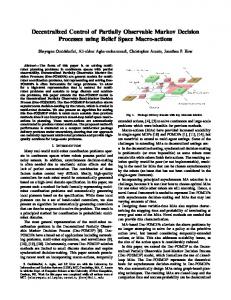
Experiments — Setup • • • •
The person walks along dash line The robot follows the people by remote-control Sick laser: 4Hz up-rate RBPF: 1000 particles
Ubot (Developed by ITRI) 14 Industrial Technology Research Institute (ITRI)
Kuo-Shih Tseng
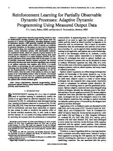
Experimental Results — Kalman filter vs. RBPF 1500
) m c( Y
1000 KF 500
RBPFT People
0 -50
0
50
100
150
200
250
-500 X (cm)
Robot position Predicted moving object of KF Corrected moving object of KF Estimated mean of moving object of RBPF Particles of moving object of RBPF Static feature
300
200
) m c( Y
KF 100
RBPFT People
0 -50
0
50
100
150
200
-100
Dynamic feature
X (cm)
15 Industrial Technology Research Institute (ITRI)
Kuo-Shih Tseng
Experimental Results — Kalman filter v.s. RBPF • Observable case Tracking standard deviation error comparison between KF and RBPF
Tracking error comparison between KF and RBPF KF RBPF
35
40 35 Standard Deviation Error
30 Tracking Error
KF RBPF
25 20 15 10
30 25 20 15 10
5
5
0
0
1
2
3
4
5
1
Experiment
2
3
4
5
Experiment
16 Industrial Technology Research Institute (ITRI)
Kuo-Shih Tseng
Experimental Results • POMOT case Tracking error comparison between KF and EBPF in POMOT case
Tracking standard deviation error comparison between KF and RBPF in POMOT case
KF RBPF
1200 Tracking standard deviation error
1800 1600 Tracking Error
1400 1200 1000 800 600 400 200
KF RBPF
1000 800 600 400 200 0
0 1
2
3
4
1
5
2
3
4
5
Experiment
Expeiment
17 Industrial Technology Research Institute (ITRI)
Kuo-Shih Tseng
Summary • Conclusions – It’s the first time that Stream field is used in object tracking – Compared with KF, Rao-Blackwellised Particle Filter (RBPF) is a good estimator for stream field based tracking.
• Future work – Considering POMOT in unknown environment.
18 Industrial Technology Research Institute (ITRI)
Kuo-Shih Tseng
Instead of guessing what the person is thinking, guessing how the person is sinking.
Thank you! ???
Stream Field for Motion Model of Tracking {
}
S k = ski , wki | 1 ≤ i ≤ N , S ik = Oki , Gki , D =
i
i
Ox , k , O y , k , Σ O , k , G x , k , G y , k , U k , D
bel (S k ) = P (S1:k | z1:k ) = P(Oki , Gki , O1i:k −1 , G1i:k −1 , D | z1:k ) = P(Gki | G1i:k −1 ) P (Oki | Oki −1 , Gki −1 , D, z k ) P (Oki −1 , Gki −1 , D | z k −1 ) 142 4 43 4 1444 424444 3 144424443 goal set sampling
objec set distribution
bel ( S k −1 )
P(Oki | O1i:k−1,G1i:k−1, D, z1:k ) 1444424444 3 objec set distributi on
=η P(zk | Oki ) P(Oki | O1i:k−1,G1i:k−1, D, z1:k−1) 1424 3 14444244443 object Correction
object Prediction
bel (S k ) = P (S1:k | z1:k ) = η P (Gki | Gki −1 ) P (Oki | O1i:k −1 , G1i:k −1 , D, z1:k −1 ) P( z k | Oki ) P(Oki −1 , Gki −1 , D | z k −1 ) 14243 14444244443 1424 3 144424443 goal set sampling
object Prediction
object Correction
bel ( S k −1 )
20 Industrial Technology Research Institute (ITRI)
Kuo-Shih Tseng
Appendix I. Stream Field for motion model of tracking {
}
S k = ski , wki | 1 ≤ i ≤ N , S ik = Oki , Gki , D =
i
i
Ox , k , O y , k , Σ O , k , G x , k , G y , k , U k , D
bel (S k ) = P(S1:k | z1:k ) = P(Oki , Gki , O1i:k −1 , G1i:k −1 , D | z1:k ) = P(Gki | Oki , O1i:k −1 , G1i:k −1 , D, z1:k ) P(Oki | O1i:k −1 , G1i:k −1 , D, z1:k ) P (O1i:k −1 , G1i:k −1 , D | z1:k ) DBN
= P ( G ki | G 1i:k −1 ) P (Oki | O1i:k −1 , G1i:k −1 , D, z1:k ) P(O1i:k −1 , G1i:k −1 , D | z1:k −1 )
markov
= P(Gki | G1i:k −1 ) P(Oki | Oki −1 , Gki −1 , D, z k ) P (Oki −1 , Gki −1 , D | z k −1 ) 142 4 43 4 1444 424444 3 144424443 goal set sampling
objec set distributi on
objec set distributi on
Doublet
bel ( S k −1 )
bel (S k ) = P(Gki | Oki ) P(Oki | Oki −1 , Gki −1 , D, z k ) P(Oki −1 , Gki −1 , D | z k −1 ) 14243 1444 424444 3 144424443 goal set sampling
D Gt −1
Gt
Sink
bel ( S k −1 )
?
Ot −1
Ot
Object position 21
Industrial Technology Research Institute (ITRI)
Kuo-Shih Tseng
Appendix I. Stream Field for sensor model of tracking bel (S k ) = P (Gki | Gki −1 ) P(Oki | Oki −1 , Gki −1 , D, z k ) P(Oki −1 , Gki −1 , D | z k −1 ) 14243 1444 424444 3 144424443 goal set sampling
=
i 1:k−1
i 1:k−1
i k
Bayes
i 1:k−1
Dt
Gt −1
Gt
Ot −1
Ot
bel ( S k −1 )
objec set distributi on
P(Oki | O1i:k−1,G1i:k−1, D, z1:k ) i k
Dt −1
i 1:k−1
i k
i 1:k−1
i 1:k−1
P(O ,O ,G , D, z1:k−1 | zk ) P(zk | O ,O ,G , D, z1:k−1)P(O ,O ,G , D, z1:k−1) = P(O1i:k−1,G1i:k−1, D, z1:k−1 | zk ) P(O1i:k−1,G1i:k−1, D, z1:k−1 | zk )P(zk )
P(zk | Oki )P(Oki ,O1i:k−1,G1i:k−1, D, z1:k−1) P(zk | Oki )P(Oki | O1i:k−1,G1i:k−1, D, z1:k−1) = = P(O1i:k−1,G1i:k−1, D, z1:k−1, zk ) P(zk | z1:k−1)
DBN
=η P(zk | Oki ) P(Oki | O1i:k−1,G1i:k−1, D, z1:k−1) 1424 314444244443 objectCorrection
z
objectPrediction
bel (S k ) = P (S1:k | z1:k )
o t
= η P (Gki | Gki −1 ) P (Oki | O1i:k −1 , G1i:k −1 , D, z1:k −1 ) P( z k | Oki ) P(Oki −1 , Gki −1 , D | z k −1 ) 14243 14444244443 1424 3 144424443 goal set sampling
object Prediction
object Correction
bel ( S k −1 )
22 Industrial Technology Research Institute (ITRI)
Kuo-Shih Tseng
Appendix II. Localization and POMOT X k = rk , S ik =
i
i
rx ,k , ry ,k , rθ ,k , Σ r ,k , Ox ,k , Oy ,k , Σ O ,k , Gφ ,k ,U k , D
bel ( X k ) = P( X1:k | u1:k , z1:k ) = P (Oki , O1i:k −1 , Gki , G1i:k −1 , rk , r1:k −1 D | u1:k , z1:k ) = P (Gki | Oki , O1i:k −1 , G1i:k −1 , rk , r1:k −1 , D, u1:k , z1:k ) P(Oki | O1i:k −1 , G1i:k −1 , rk , r1:k −1 , D, u1:k , z1:k ) P(rk | O1i:k −1 , G1i:k −1 , r1:k −1 , D, u1:k , z1:k ) P(O1i:k −1 , G1i:k −1 , r1:k −1 , D | u1:k , z1:k ) DBN
= P (Gki | G1i:k −1 ) P (Oki | O1i:k −1 , G1i:k −1 , D, rk , u1:k , z1:k −1 ) P(rk | r1:k −1 , D, u1:k , z1:k ) P (O1i:k −1 , G1i:k −1 , r1:k −1 , D | u1:k , z1:k ) 142 4 43 4 14444442444444 3 144424443 1444442444443 goal set distribution
object set distribution
bel ( X k −1 )
robot distribution
= η P(Gki | Gki −1 ) P ( z kO | Oki ) P(Oki | O1i:k −1 , G1i:k −1 , D, r1:k ) P ( z kL | rk ) P(rk | r1:k −1 , u1:k , z1:k −1 ) P (O1i:k −1 , G1i:k −1 , r1:k −1 , D | u1:k , z1:k ) 14243 14243 14444244443 1424 3 144424443 1444442444443 goal set distributi on object Correction
object Prediction
Object tracking
Robot Correction
Robot Prediction
bel ( X k −1 )
Robot localization
Obstacle Stream line
Object
Robot Industrial Technology Research Institute (ITRI)
Kuo-Shih Tseng
Sink
23
Stream Field for Motion Planning (1/2) (S. Waydo and R.M. Murray, 2003) ( x , y ) Robot position ( xd , yd ) Obstacles position Stream Field ( xs , ys ) Goal position ψ ( x, y )
time : t
Xd
Xe
+
Controller
∂ψ ( x, y ) Desired velocity of robot ∂y ∂ψ ( x, y ) Xd v=− ∂x
u=
Robot Plant
Xr
-
Robot Trajectory Industrial Technology Research Institute (ITRI)
Kuo-Shih Tseng
24