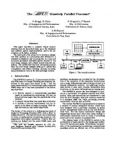
This paper describes a memory-based SIMD shared-bus parallel processor architecture, which is called âFunctional Memory Type Parallel Processorâ ...
A Study of the Functional Memory Type Parallel Processor
http://www.tamaru.kuee.kyoto-u.ac.jp/fmpp/
Kazutoshi Kobayashi Kyoto University
September 1998
Abstract This paper describes a memory-based SIMD shared-bus parallel processor architecture, which is called “Functional Memory Type Parallel Processor” abbreviated as FMPP. The FMPP architecture integrates memory and an ALU closely on a single die. All the PEs are connected with a shared bus and laid out in a two-dimensional array like memory and perform the same instructions according to the SIMD manner. The FMPP architecture enables massively parallel computing inside a memory. It has a capability to break the Von Neumann bottleneck where the system performance is limited by the bus performance between memory and CPU. We have developed four LSIs based on the bit-parallel block-parallel architecture, where a PE consists of several words and a bit-parallel ALU. The first LSI called the BPBP-FMPP with 8 PEs is designed and fabricated for general purpose. A PE consists of 32bit CAM words and a 32bit ALU for numerical and logical operations. The following three LSIs called FMPP-VQ are for a special purpose: vector quantization (VQ). A PE consists of 16 words of 8bit SRAMs and a 12bit ALU. The FMPP-VQ accelerates the nearest neighbor search where the vector nearest to an input is extracted among large number of code vectors. The FMPP-VQ4 with 4 PEs is an evaluation LSI to confirm functionalities. The second FMPP-VQ64 integrates 64 PEs. It performs over 50,000 nearest neighbor searches per second, while its power consumption is 20mW. It can be used for real-time low-rate video compression. The third FMPP-VQ64M is designed for more powerful and low-power computation. Its performance becomes almost twice, while its power consumption is half compared with the FMPP-VQ64. We have also developed a low-rate video compression system using the FMPP-VQ. The proposed multi-stage hierarchical vector quantization algorithm can transmit 10 QCIF frames per second through a 29.2kbps mobile channel.
ii
Contents 1
Introduction
1
2
Overview of Parallel Processor and Functional Memory
3
2.1
3
2.2
2.3 3
3 5 7 7 9 10 13
Functional Memory Type Parallel Processor: FMPP
15
3.1
15
3.2 3.3
3.4
3.5 4
������ 2.1.1 Von Neumann Computer Architecture ������������������� 2.1.2 SIMD Parallel Processor to Solve the Von Neumann Bottleneck ����� Functional Memory and Associative Processor ������������������ 2.2.1 Content Addressable Memory ����������������������� 2.2.2 Associative Processors ��������������������������� 2.2.3 Implementations of Associative Processors ���������������� Summary of the Chapter ������������������������������ Parallel Processor Architectures to Break the Von Neumann Bottleneck
������������������������������� FMPP Architectures According to the PE Granuality ��������������� Implementations of the FMPP Architecture �������������������� 3.3.1 Bit-serial Word-parallel Architecture ������������������� 3.3.2 Bit-parallel Block-parallel Architecture ������������������ Parallel Computation Efficiency on the FMPP ������������������� 3.4.1 Von Neumann Bottle Neck on the Conventional Computer �������� 3.4.2 Parallel Computation on the FMPP �������������������� Summary of the Chapter ������������������������������ Features of the FMPP
17 18 19 21 25 25 27 31
An Implementation of the Bit-Parallel Block-Parallel FMPP
33
4.1
BPBP-FMPP
33
4.1.1
34
4.1.2 4.1.3 4.1.4
������������������������������������ Logical Operations on the CAM Cell ������������������� Block Diagram ������������������������������ Primary Operations ���������������������������� Data Mask and Address Mask Operations �����������������
34 35 36
iv
Contents
����������������� Detailed Operation Strategies ��������������������������� 4.2.1 Logical Operations ���������������������������� 4.2.2 Addition and Subtraction ������������������������� 4.2.3 Shift/rotate Left Operation ������������������������� 4.2.4 Search Operation ����������������������������� 4.2.5 Multiplication ������������������������������� 4.2.6 Multiple Response Resolution ����������������������� 1kbit BPBP-FMPP LSI ������������������������������ 4.3.1 LSI Overview ������������������������������� 4.3.2 Test Results �������������������������������� 4.3.3 Comparison for the Circuit Areas between CMOS and CPL Logics ���� Applications of the BPBP-FMPP ������������������������� 4.4.1 Threshold Search and Extremum Search ����������������� 4.4.2 Knapsack Problem ����������������������������� Summary of the Chapter ������������������������������ 4.1.5
4.2
4.3
4.4
4.5
Detailed Structure of the Memory Block
5 Functional Memory Type Parallel Processor for Vector Quantization: FMPP-VQ 5.1 5.2 5.3 5.4
5.5
5.6
������������������������������������ Vector Quantization of Image ��������������������������� Vector Quantization on the FMPP ������������������������� Architecture and Structure ����������������������������� 5.4.1 Nearest Neighbor Search on the FMPP-VQ ���������������� 5.4.2 Structure of the FMPP-VQ ������������������������ 5.4.3 Detailed Structure of the PE ������������������������ 5.4.4 Nearest Neighbor Search Procedure �������������������� 5.4.5 List of Operations on the FMPP-VQ �������������������� Implementations of FMPP-VQ LSIs ������������������������ 5.5.1 An LSI Including Four PEs and TEGs: FMPP-VQ4 ������������ 5.5.2 An LSI Including 64 PEs and Control Logics: FMPP-VQ64 ������� 5.5.3 Integration Density of the FMPP-VQ64 ������������������ 5.5.4 Testability of the FMPP-VQ64 ���������������������� Modified Version of the FMPP-VQ: FMPP-VQ64M ���������������� 5.6.1 Structure of a PE ������������������������������ 5.6.2 Absolute Distance Computation ���������������������� Introduction
37 38 39 39 41 41 41 43 43 43 44 45 46 47 48 49 51 51 53 55 56 57 58 60 67 68 72 72 73 76 77 78 79 80
Contents
v
����������������������� 5.6.4 A Highly-Functional Control Logic �������������������� 5.6.5 Specification and Implementation ��������������������� Comparison with Other Implementations ��������������������� 5.7.1 Comparison with the Other Vector Quantizer. ��������������� 5.7.2 Comparison with the Von Neumann Sequential Processors. �������� 5.6.3
5.7
5.7.3
5.8
5.9 6
Detailed Structure of the ALU
Comparison with an Application Specific Processor for Vector Quantization
�� 5.8.1 Overview of the Real-Time Low-Rate Video Compression System ���� 5.8.2 Coding Algorithm ����������������������������� 5.8.3 Experimental Real-Time Low-Rate Video Compression System ����� 5.8.4 Performance Evaluation �������������������������� Summary of the Chapter ������������������������������ A Low-rate and Low Power Image Compression System Using the FMPP-VQ
Conclusion
81 83 84 88 88 92 93 95 96 97 102 104 109 111
Bibliography
114
Publication List
121
Acknowledgment
125
vi
Contents
List of Figures 2.1 2.2 2.3 2.4 2.5 2.6 2.7 2.8 2.9 2.10 3.1 3.2 3.3 3.4 3.5 3.6 3.7 3.8 3.9 3.10
���������� IMAP LSI. ������������������������������������� Block diagram of a 4kb CAM. ��������������������������� Memory cells of a CAM(left) and a conventional 6-transistor SRAM(right). ��� Match line on a CAM cell. ����������������������������� General bit-serial associative processors. ��������������������� Multiple-valued CAM cell. ���������������������������� A pixel parallel image associative processor[HS92, GS97]. ������������ Dynamic content addressable memory cell. �������������������� An implementation of computational RAM. �������������������� Von Neumann computer and its hierarchical memory structure.
�������������� Several FMPP architectures according to PE granuality. �������������� Flow chart of the minimum value search. ��������������������� Procedure for the minimum value search. ��������������������� Threshold search on CAM. ���������������������������� Algorithm for global addition. ��������������������������� Data flow-chart of global addition. ������������������������� Algorithm for local addition. ���������������������������� Data flow-chart of local addition. ������������������������� Whole structure of the functional memory for parallel addition. ���������� Functional memory type parallel processor architecture.
4 6 8 9 9 10 11 11 12 12 16 17 19 19 20 21 21 22 22 23
3.11 Processing element of the functional memory for parallel addition(a), its memory cell
����������������������������������������� Layout pattern of a PE. ������������������������������� Structure of the FMPP-IP. ����������������������������� Processing Unit of the FMPP-IP. �������������������������� Processor DRAM gap[Fro98]. ��������������������������� A computer system using an FMPP as a part of main memory. ���������� Total execution time on the Von-Neumann computer and on the FMPP. ������ (b).
3.12 3.13 3.14 3.15 3.16 3.17
23 24 24 24 25 27 28
viii
List of figures
������� Performance efficiency of an Neumann Computer system / an FMPP system. ���
3.18 Von Neumann system with cache memory and FMPP-based system.
29
3.19
30
4.1 4.2 4.3 4.4 4.5 4.6 4.7 4.8 4.9 4.10 4.11 4.12 4.13 4.14 5.1 5.2 5.3 5.4 5.5 5.6 5.7 5.8 5.9 5.10 5.11 5.12 5.13 5.14 5.15 5.16 5.17 5.18
������������������������� Block diagram of the BPBP FMPP LSI. ���������������������� Structure of a PE. ��������������������������������� Detailed schematic structure of a memory block. ����������������� An FMPP memory cell and logical operations. ������������������ The buffers P & G. ��������������������������������� Manchester carry chain. ������������������������������ Addition between 2 words. ����������������������������� Multiplication between 2 words. �������������������������� Layout pattern of a four-bit slice of the memory block. �������������� Chip micro photograph of the BPBP-FMPP. �������������������� Operating waveforms from read/write operations. ����������������� Computation time of extremum search. ���������������������� Computation time of knapsack problem. ���������������������� Logical operations on a CAM cell.
��������������������������� Nearest neighbor search and codebook optimization. ��������������� Block diagram of the FMPP-VQ. ������������������������� Structure of a PE. ��������������������������������� Layout pattern of a PE. ������������������������������� One bit slice of the ALU. ����������������������������� Operand word. ����������������������������������� Search line and reference line for the search operation. �������������� Two bit slice of the carry chain. �������������������������� Inverter controlled by an NMOS FET. ����������������������� XNOR (exclusive-nor) gate. ���������������������������� Temporary word. ���������������������������������� Result word. ������������������������������������ Schematic view of two flags. ���������������������������� The overflow flag and the part of the local control logic. �������������� Column priority address encoder. ������������������������� Two dimensional priority address encoder for the FMPP-VQ64. ���������� Procedure for computing the absolute distance. ������������������ Vector quantization of images.
34 35 36 38 38 39 39 40 42 44 46 47 48 49 54 55 58 60 60 61 61 61 62 62 62 63 63 64 64 65 66 68
List of figures
ix
���������������������� The minimum value search procedures. ���������������������� Timing Diagram of the FMPP-VQ. ������������������������ Whole procedure to perform the nearest neighbor search. ������������� Chip microphotograph of the FMPP-VQ4. ��������������������� The detailed block diagram of the FMPP-VQ64. ������������������ Verilog-HDL description of the operand word and the carry chain. �������� The chip microphotograph of the FMPP-VQ64. ������������������ A measured Shmoo plot of supply voltage versus cycle time in the FMPP-VQ64. � Dynamic Current flow on the absolute distance computation. ����������� Parallel random-access capability to the ALU. ������������������� PE structures of the FMPP-VQ64(a) and the FMPP-VQ64M(b). ���������
5.19 Program of the minimum value search.
69
5.20
69
5.21 5.22 5.23 5.24 5.25 5.26 5.27 5.28 5.29 5.30
71 71 73 74 75 76 77 78 79 80
5.31 A single dimension slice of the absolute distance computation in FMPP-VQ64M.
82
5.32 Two-bit slice of the ALU.
83
5.33
84
5.34 5.35 5.36 5.37 5.38 5.39 5.40 5.41 5.42 5.43 5.44 5.45 5.46 5.47 5.48 5.49 5.50 5.51
����������������������������� Structure of the operand word. ��������������������������� Inverter controlled by a PMOS FET. ������������������������ Structure of the result word. ���������������������������� The flow of mode changes in the FMPP-VQ64M. ����������������� Layout of a PE. ���������������������������������� Chip micrograph of the FMPP-VQ64M. ���������������������� A systolic binary-searched vector quantizer. �������������������� A systolic full-searched array processor[WC95]. ����������������� A serial full-searched MSE processor[CWL96] . ����������������� � A fully-parallel 256-elements parallel processor[SNK 97] . ������������ C � RAM implementation of vector quantization for video compression[LP95]. �� C program for the nearest neighbor search. �������������������� The assembler program to compute the absolute distance of a single dimension. � An application specific processor for VQ. ��������������������� Schematic diagram of the low-rate video compression system. ���������� Four hierarchical stages for decimation and interpolation. ������������� Block diagram of our coding algorithm. ���������������������� Derivative code vectors from a primitive vector. ������������������ Experimental real-time low-rate video compression system. ������������
84 84 84 87 87 89 90 91 91 92 93 94 95 96 98 99 101 104
5.52 Computation amount of each function on decoding of the fixed-rate MSHVQ and H.263.
���������������������������������������
104
x
List of figures
�������� Temporal bit allocation of Suzie for the proposed MSHVQ algorithm and H.263. � PSNR transitions from High Random BER (10 � 3 ) using Mother&Daughter. ��� PSNR transitions from Multiple Burst Errors using Mother&Daughter. ������
5.53 PSNRs of the proposed MSHVQ algorithm and H.263 for “Suzie.”
105
5.54
105
5.55 5.56
107 107
List of Tables 2.1
SIMD distributed-memory parallel processor implementations.
3.1
Parameters for a conventional Von Neumann computer.
����������
3.3
�������������� Spec of Portege 620CT. ������������������������������ Parameters to compare a Neumann Computer system with an FMPP system. ���
4.1
Primary operations on the BPBP-FMPP.
3.2
4.2 4.3 4.4
���������������������� Overview of the 1kbit BPBP-FMPP LSI. ��������������������� Component areas of the 1kbit FMPP LSI together with a 256kbit SRAM. ����� Comparison of the structure for logical operation. �����������������
5.5
����������������� All available SIMD operations of the FMPP-VQ. ����������������� Other operations of the FMPP-VQ. ������������������������ LSI specifications of the FMPP-VQ4. ����������������������� LSI specifications of both of the FMPP-VQ4 and FMPP-VQ64. ����������
5.6
Comparisons of power dissipation by activating the inverter at the numerical operation
5.1 5.2 5.3 5.4
Parameters and definition for vector quantization.
�������� Area for 1 PE of the FMPP-VQ64 and 8kbit SRAM fabricated by the same 0.7� m process. �������������������������������������� and by always activating the inverter. The condition is 5V/25MHz.
5.7
5.8
Comparison of areas and performance for the FMPP-VQ64 and the FMPP-VQ64M.
5.9
Power consumption of the FMPP-VQ64M from circuit simulations of a PE at 25MHz
���������������������������������������� Power dissipation map for all the components in a PE. �������������� 5.0V.
5.10
6 26 26 30 37 45 45 46 56 70 70 72 74
76
77 85
85 86
5.11 The power consumption of the FMPP-VQ64M expected from the measured results
�������������������������������� Areas for PEs of the FMPP-VQ64 and FMPP-VQ64M. �������������� The areas for FMPP-VQ64 and FMPP-VQ64M. ������������������ Number of standard cells for control logics. �������������������� Comparison with the other vector quantizers. ������������������� of the FMPP-VQ64.
5.12 5.13 5.14 5.15
86 86 87 88 92
xii
List of figures
5.16 Speed and power dissipation table of the nearest neighbor search among 64 code
��������������������������������������� SRAM specifications. ������������������������������� Contents of compressed 2920bit data. ����������������������� Average PSNRs for 8 standard video sequences. ������������������ Error conditions[MPE95]. ����������������������������� vectors.
5.17 5.18 5.19 5.20
93 94 103 106 107
5.21 Average PSNRs from High Random BER (HRB) and Multiple Burst Errors (MBE) conditions.
�������������������������������������
108
Chapter 1 Introduction This paper is a summary of a memory-based SIMD (single instruction multiple data stream) sharedbus parallel processor architecture, which is called the “Functional Memory Type Parallel Processor” abbreviated as FMPP. Almost all the current computing systems are based on the Von Neumann architecture, where a CPU and memory devices are connected with a shared bus. All the data and programs should be transfered between the CPU and memory through the bus. Although the performance of the CPU is rapidly improving, the performance of the Von Neumann system is limited by the performance of the bus or the memory, which phenomenon is called “Von Neumann Bottleneck.” This is because the performance of the memory is not improved faster than that of the CPU and the width of the bus is limited to be narrow. The bottleneck must be alleviated to perform processing inside a memory device. The memory device implies parallel computation capability, since it consists of a two-dimensional array of memory words. All the words can work in parallel. The two-dimensional regular array structure achieves highly dense layout improving four times every three years. The FMPP architecture allows parallel processing inside memory devices. A processing element (PE) consists of some amount of memory cells and an ALU. All the PEs connected with a shared-bus work in parallel according to a single instruction provided through a central control unit (the SIMD control method). The FMPP is suitable for operations where communication between processors or external devices is not so frequent and the same operations are done for huge number of data set. The processing capability is defined by the processor granuality. Fine granuality makes the functionality poor. Coarse granuality enlarges the area. A bit-parallel block-parallel (BPBP) structure is proposed in this paper for middle-grain modest-functional processing. The PE consists of several words and a bit-parallel ALU. Four LSIs have been developed and fabricated based on the BPBP structure. The first emerged LSI is called BPBP-FMPP, which contains eight 32bit PEs and can be applied for general purpose. The following three LSIs called the FMPP-VQ are for a special purpose: vector quantization (VQ). A PE consists of 16 eight-bit SRAMs and a 12bit ALU. The FMPP-VQ can search the vector (pattern) nearest to an input among all the vectors stored in PEs. It is successfully applied to real-time low-rate video compression by VQ. The first FMPP-VQ LSI
2
Chapter 1. Introduction
contains four PEs to evaluate its functionalities. The second and third attempts integrate 64 PEs to be applied for real-time low-rate image compression. We have also developed an algorithm and a real-time low-rate compression system using the FMPP-VQ. Chapter 2 gives overview of the functional memory. The functional memory is a memory device with some functionalities. The FMPP can be categorized to the functional memory. The CAM and associative processor architectures are also discussed. Chapter 3 explains the FMPP architecture in detail. The BPBP structure is compared with the other two structures, bit-parallel word-parallel and bit-serial word-parallel. The performance efficiency on the FMPP-based computing system is also argued. The BPBP-FMPP is described in Chapter 4. Chapter 5 introduces the FMPP-VQ architecture, the three LSI implementations and the real-time low-rate video compression system. Chapter 6 summarizes this paper.
Chapter 2 Overview of Parallel Processor and Functional Memory This chapter describes the overview of parallel processor and functional memory. The functional memory type parallel processor (FMPP) is a parallel processor architecture based on functional memory. First, we address the Von Neumann bottleneck eliminating the performance of the current computing system. Several parallel processor architectures are introduced to break the bottleneck. Then, functional memory and associative processors are described in detail.
2.1 Parallel Processor Architectures to Break the Von Neumann Bottleneck The current Von Neumann computer architecture confronts the bottleneck where the system performance is limited by the bus performance. This section gives the brief description of the bottleneck and shows several parallel processor architectures to break the bottleneck.
2.1.1 Von Neumann Computer Architecture In the Von Neumann architecture, computers are composed of a central processing unit (CPU) and a memory unit (Figure 2.1). CPU performs operations according to codes (programs) and data in the memory unit. They are connected with a bus. At the rise time of computers, thousands of relay switches and vacuum tubes form a computer unit. As the emergence of semiconductor devices, the memory and CPU are replaced with discrete transistors. Now they are integrated on LSIs (Large Scale Integrations or Large Scale Integrated circuits). The most popular commercial processor Pentium integrates over 1 million transistors and its internal clock speed becomes over 300MHz. The largest commercial DRAM (Dynamic Random Access Memory) has 256 million bits on a single LSI. In the Von Neumann architecture, all data and codes have to be passed from the main memory to the CPU through the bus. The bandwidth between them is narrow, since the number of pins pulled outside LSIs are limited. Pentium has only 64-bit bus. The access time of DRAM is about 50ns
4
Chapter 2. Overview of Parallel Processor and Functional Memory
(20MHz). In these conditions, Pentium can perform 300MIPS (Mega instructions per second), but the DRAM gives only 160M bytes of data and codes per second to the CPU. The bus degrades the performance of the CPU, which is so-called “Von Neumann bottleneck.” To compensate the Von Neumann bottleneck, all of current commercial CPUs have memory hierarchy as shown in Figure 2.1. The memory hierarchy virtually shortens the access time of the DRAM if the accessed data exists on cache memory (Cache Hit). The actual access time, however, becomes longer because the actual distance from the CPU to the DRAM becomes longer. That produces severe problems in some applications. For example, these hierarchical structure of cache memory is not so effective for image processing. Image processing usually applies the same operations to image data. The image data of video sequence amounts to huge size. In the JPEG, the famous DCT-based image compression algorithm, the image data is divided into a block, each of which includes 8 � 8 pixels. Each block has no relation with others. In this situation, the first cache in the CPU can store a single block data, which accelerates processing. But the second cache between DRAM and CPU does not contribute the processing speed. It merely prolongs the access time of DRAM.
$
CPU
$ bus
2nd Cache
ALU
1st Cache
register files
Main Memory
(DRAM)
bus
$
HDD
$
HDD
bus
$=cache
Figure 2.1: Von Neumann computer and its hierarchical memory structure.
As for the power dissipation, an off-chip bus to connect the CPU and memory dissipates a large amount of power. Reference [Wat98] mentions that an external pin-to-pin I/O connection yields 50pF of stray capacitance, while an internal I/O connection yields only 1pF which is 50 times smaller. The dissipated power is proportional to the value of stray capacitance. If we implement the CPU and memory in a single LSI, the power dissipation must be minimized. Recently, such a challenge called “Merging memory (DRAM) and Logic” becomes very popular. The deep sub-micron process on the current VLSI technology actualizes a mixture of logic and DRAM on a single LSI. Some
�
LSI vendors develop commercial products implementing some amount of DRAM and logics on
�
�
a single die[INK 95, WFY 97]. eRAM
by Mitsubishi Electric Corp. stands for “embedded
�
random access memory”[ERA]. The 3D-RAM[INK 95] is one of LSIs of the eRAM architecture. It integrates Z-compare or -blend units to be applied to 3D-graphic applications. A single LSI
contains 10Mbit DRAM and an SRAM cache with a single ALU for Z-compare or -blend. Several
2.1. Parallel Processor Architectures to Break the Von Neumann Bottleneck
5
LSIs simultaneously work to complete 3D-graphic applications.
2.1.2 SIMD Parallel Processor to Solve the Von Neumann Bottleneck Several approaches can be taken to break the Von Neumann bottleneck. One approach is to have multiple CPUs work in parallel, which is called “parallel processors.” Pentium now integrates SIMD processors, which is called MMX extension, which is suitable for image processing or video game. Parallel processor is a key technology to obtain more powerful and effective computation on LSIs. Parallel processor is categorized in two by its memory architecture: distributed memory and shared memory. In the distributed memory architecture, a processor has its own memory, while all the processors shares common memory in the shared memory architecture. The distributed alleviates the bottleneck more than the shared, since the bandwidth between memory and processor is extended according to the number of processing elements (PEs). A complex control method usually makes it difficult to describe a parallel program and makes the area of the PE larger. General parallel processors can also be grouped into two major categories by the control method. One is SIMD that means “Single Instruction Multiple Data Stream.” The other is MIMD that is an abbreviation of “Multiple Instruction Multiple Data Stream.” On the SIMD, all processors work simultaneously according to the same instruction. On the MIMD, each processor performs its own instruction. An SIMD parallel processor can be implemented in a smaller area than an MIMD parallel processor, since a PE of the MIMD should have its own control logic. All PEs of the SIMD, however, can be controlled by a common control logic. The number of PEs on a single die should become larger in the SIMD architecture. Thus, the SIMD distributed-memory parallel processor is a good candidate to break the bottleneck. We should consider some more parameters to implement SIMD distributed-memory parallel processors. Here, these three parameters are chosen to categorize them : processor granuality, processor functionality and communication network. They have strong correlation with each other. Fine processor granuality usually makes the functionality of a PE poorer. Complex communication network always makes the area of an LSI larger. We introduce several implementations of SIMD distributedmemory parallel processors by those three parameters. Table 2.1 shows the three implementations of the SIMD distributed-memory parallel processors. Connection Machine[Hil87] is an SIMD parallel processor. In the first system called CM1, each PE consists of 4kbit memory and a bit-serial ALU, which is very simple. The CM1 consists of 64k PEs connected with a complex flexible network called “hyper-cube.” A software programmer can design a network of processors as he want. Connection Machine is developed for general purpose. Content Addressable Memory (CAM) is a memory device which can associate address from contents of memory. Detail descriptions are shown later in Section 2.2.1 and Section 3.3.1. It is
6
Chapter 2. Overview of Parallel Processor and Functional Memory
Table 2.1: SIMD distributed-memory parallel processor implementations. Granuality Functionality Network (Type) Connection Machine
fine
poor
Complex (Hyper-cube)
CAM
very fine
very poor
Simple (Bus-connected)
IMAP
coarse
medium
Simple (Bus-connected)
usually regarded as memory than parallel processors. But it can be applied to parallel processing using its associative capability as shown in Section 3.3.1. IMAP stands for Integrated Memory Array Processor proposed by a group of NEC[FYO92]. It
�
is an SIMD parallel processor architecture merging SRAM and logic. The IMAP LSI[KNA 95] integrates a 2MB SRAM with 64 PEs. The block diagram is shown in Figure 2.2. A 64kb SRAM macro is assigned to two PEs. They can directly communicate with the assigned SRAM macro.1 Each PE consists of several 8bit registers and an 8bit ALU. Its peak performance becomes 3.84 GIPS, but its power consumption is 4W. An image processing system connected to the PCI bus is already commercially available[NEC].
64kb SRAM x 10
Main Bus
Memory Bus
PEx16
64kb SRAM x 10
Figure 2.2: IMAP LSI.
As described above, various distributed-memory SIMD parallel processor architectures are available. In the Connection Machine architecture, complex network reduces the integration density. The 1
8 SRAM macros are redundant.
2.2. Functional Memory and Associative Processor
7
progress of the current VLSI technology enlarges the integration density year by year. The memory device enjoys the progress enormously, since its two-dimensional array structure and shared-bus simple network are very much suited to the VLSI technology. Thus, the parallel processor architecture based on the memory structure may hugely enjoy the VLSI technology. The CAM has the capability to perform parallel processing inside memory. But its functionality is too poor. The IMAP integrates multiple processor and memory devices on a single die. But memory and processor are separately designed and the processor granuality is relatively coarse. In this paper, we focus on a memory-based SIMD shared-bus parallel processor architecture called FMPP. FMPP stands for Functional Memory type Parallel Processor. The FMPP architecture enables fine-grain highly-functional parallel processing inside memory. It allows numerical operations inside memory. In the next section, we introduce functional memory and associative processor before describing the FMPP architecture.
2.2 Functional Memory and Associative Processor Functional memory can be described as a memory including some simple functions such as content addressing. It is proposed by Kohonen[Koh87] as “associative memory.” The original associative memory is some kind of conceptual one. It can associate a target value from several key values like our brain. Kohonen implemented an optical associative memory to retrieve a full-sized image from an incomplete image. On the other hand, content addressable memory (CAM) is an actual LSI implementation of associative memories. Conventional memories like DRAMs or SRAMs associate data from an address, while the CAM associates an address from data. Associative processor is a parallel processor architecture to perform processing using its associativity. Here we explain the CAM and the associative processor in detail. Implementations of the FMPP proposed in this paper are based on the CAM architecture.
2.2.1 Content Addressable Memory Ogura et al. implemented a 4kb content addressable memory[OYN85] in early 80’s as shown in Figure 2.3. Its memory cell is shown in Figure 2.4 along with a memory cell of a conventional 6-transistor SRAM. The two pass transistors denoted by dashed circles work as a pass-transistored XNOR (exclusive-nor) logic. Let the CAM cell store � and supply and b1 respectively. Note that the supplied value is inversed: b0 �
�
becomes logic high if
�����
1 � & ����� 0 � or
�����
�
�
and �
to the two bit lines b0
and b1 ��� . The output node
0 � & ����� 1 � . It means ����� (XOR). To obtain
words matched to a key value, the multiple bits of a CAM cell form a single match line that works as a wired-NOR of all results from the XOR gates (See Figure 2.5). In the initial condition, the Match
8
Chapter 2. Overview of Parallel Processor and Functional Memory
line is precharged. A key value is supplied to the CAM word, then the
� ��!
is activated. If
�"�#�
,
the match line keeps logic high, or it is discharged since an XNOR gate where �%$'&)(+�� * �,$ &)( becomes true. The search flag connected to the Match line stores the search result. We call the operation “search operation.” The search operation may have multiple search flags become true. The multiple response resolver resolves the lowest address among CAM words search flags of which are true. The signal -/. becomes false if there is no true search flag. The garbage flag invalidates the search result. It is usually used to read all the addresses search flags of which are true. When the lowest word (the word address of which is the lowest of all) is read out, its garbage flag becomes true. Then, the multiple response resolver produces the second-lowest address. Such an operation is called “Multiple Response Resolution.” The CAM also has a functionality of parallel write operation: writing all the words whose search flags are true.
key
Search flag
CAM Word
Garbage flag
Match
CAM cell
CAM cell
Match line
CAM cell Match
Match
CAM Cell Array
CAM cell
CAM cell
CAM cell
Multiple Response Resolver
mask registers
Associated Address ER
Figure 2.3: Block diagram of a 4kb CAM.
The mask register located at the top of the CAM cell array in Figure 2.3 masks specified bits. The two bit line b0 and b1 become logic low at the masked bit. Thus, the XNOR gate of the bit always generates the false output regardless of the bit data. Thus, the specified bit is masked on the search operation. The mask signal in the CAM cell is also connected to the mask register. It is used to prohibit the write operation to the specified bit. They applied the CAM to Prolog machines[NO90]. The CAM accelerates the back-track scheme. The garbage flags support the garbage collection in Prolog. They have been developing high-density
�
CAM LSI implementations[FOT93, ONB 96, ON97]. The latest CAM LSI in [ON97] integrates
2.2. Functional Memory and Associative Processor
9
mask B
B
b1
b0
b1
b0
W
W
A
A
Match
Match C
Match
Match
Figure 2.4: Memory cells of a CAM(left) and a conventional 6-transistor SRAM(right).
bit1[m:0] bit0[m:0]
B A
mbit CAM word
CAM Cell
CAM Cell
CAM Cell
PRE
Match
bit0
bit1
bit2
Match
Match bitm Match
Figure 2.5: Match line on a CAM cell. 366k-bit on a 16.5 � 16.5 mm2 die, which is applied to image processing.
2.2.2 Associative Processors S.S. Yau and H.S. Fung surveyed associative processors in Reference [YF77]. An associative processor can generally be described as a processor which has the following two properties: 1. Stored data items can be retrieved using their content or part of their content (it is called content addressing). 2. Data transformation operations both arithmetic and logical can be performed over many sets of arguments with a single instruction (it is called parallel computation). Although, the CAM has only the former property, we can regard the CAM as an associative processor. Almost all implementations to be categorized into associative processors are based on the content addressing capability of the CAM. In the rise time of associative processors, they were applied to various fields, for example, geometrical problems[SKO90], a database accelerator[WS89],
10
Chapter 2. Overview of Parallel Processor and Functional Memory
a Prolog engine[NO90] and etc. But current target applications tend to image processing. This may be because advantages obtained by these embedded associative processors are soon supposed by commercial micro processors which have remarkably been improving. In the area of image processing, however, these associative processors get a great advantage over the micro processors on the processing speed and power dissipation. The architecture of associative processors can generally be classified into three categories according to the processor granuality. The three categories are bit-oriented, word-oriented, and blockoriented associative processors. The bit-oriented associative processors is the most fine grain one, which PE consists of a single-bit memory cell with an ALU. A single word with an ALU forms the PE of the word-oriented associative processors. The block-oriented associative processors are implemented as the bit-parallel block-parallel FMPP in this paper. It consists of several words of memory cells and an ALU. Comparison of these three architectures is discussed in Section 3.2. The word-oriented architecture is the most widely-spread and famous, since it can easily be implemented to add a specific word-oriented ALU to a CAM word as shown in Figure 2.6. The ALU retrieves the single bit data through the match line of a CAM word.
Word-oriented Logic Unit
CAM Array 1word=1PE
Figure 2.6: General bit-serial associative processors.
2.2.3 Implementations of Associative Processors Here, several implementations of associative processors are introduced. A group of Waseda University[Was] proposed a CAM-based hardware engine for geometrical
�
problems[KNK 92]. They developed a 4kbit CAM to accelerate threshold search, extremum search and parallel numerical operations. Numerical operations are done in bit-serial in an ALU attached to a word. A group of Tohoku University[Toh] develops a multiple-valued CAM [HAK97]. A cell of the CAM is a floating-gate MOS transistor similar to EEPROM cells (Figure 2.7). The floating-gate MOS
2.2. Functional Memory and Associative Processor
11
transistor stores 4 states by controlling the threshold voltage. They just propose a circuit diagram of the CAM. They will apply it to fully parallel template-matching operations. They carry out another research of intelligent vehicles, where a ROM-type CAM is applied to collision avoidance[HK96]. Digit line Match line Floating gate Word line
Figure 2.7: Multiple-valued CAM cell.
A dynamic associative memory processor has been proposed by Sodini et. al. in [HS92]. As shown in Figure 2.8 a two-dimensional network connects all the PEs. A PE consists of associative parallel processors which can be word-oriented or fully-parallel. A memory cell is called a dynamic contentaddressable parallel processor cell as shown in Figure 2.9. Image processing such as smoothing is introduced as an effective application on the dynamic associative memory processor, with each PE assigned to a single pixel. They fabricated a 256-element associative parallel processor LSI[HS95]. Currently, they have proposed and fabricated a pixel-parallel image processor based on the DRAMmerged logic architecture[GS97]. A PE has the similar structure in the dynamic associative memory processor. But a memory cell is replaced with a conventional DRAM cell. It integrates 128 � 128 processors on a 78.6mm2 die.
Associative processor array Analog-to-digital converter Imager
Analog Processor
PE Processing element
PE
PE
PE
PE
PE
PE
PE
PE
PE
Host computer
Figure 2.8: A pixel parallel image associative processor[HS92, GS97].
Processed images out
12
Chapter 2. Overview of Parallel Processor and Functional Memory
Match MD MS0
MS1
Write word
MW0
MW1
B0
B 1 Write trit
Figure 2.9: Dynamic content addressable memory cell.
Computational RAM (C � RAM ) is a memory-SIMD hybrid architecture where each column of memory has an associated processing element[ESS92]. Figure 2.10 shows an implementation of C � RAM. There are 64 bit-serial PEs. A 1kbit memory column is assigned to each PE. It is applied to several image processing application including vector quantization. The detail description of applying vector quantization is explained in Section 5.7 compared with the implementation of the FMPP.
memory column
PE
PE
PE
PE
PE
PE
instruction data
64
memory column
63
memory column
4
memory column
3
memory column
bit-serial
2
memory column
address
row decoder
1
broadcast bus
Figure 2.10: An implementation of computational RAM.
2.3. Summary of the Chapter
13
2.3 Summary of the Chapter Here, parallel processor and functional memory are briefly discussed. Von Neumann architecture has been used in the current computer system. At the emergence of the computer, the CPU and the memory are separately fabricated. But now both can be integrated on a single die. The challenge to merge memory devices and processors on a single LSI has just started recently owing to the current rapid progress of integration density. It extends the bandwidth between memory and processors considerably. But the speed gap between DRAMs and processors still remains. The gap should be compensated by memory hierarchical structure. But it prolongs the bus length. If some amount of processing can be done on memory devices, the system performance will be promoted. The functional memory architecture attaches simple processing capability to memory devices to enable on-memory processing. The CAM, the most famous widely-used functional memory can detect an address from its content. It can be regarded as a parallel processor where each word becomes a processor. Its two-dimensional structure is very much suited to the current VLSI technology. The functional memory type parallel processor, FMPP architecture described in the next chapter can be categorized to the functional memory. It is a memory-based SIMD shared-bus parallel processor. The FMPP integrates fine-grain memory-based PEs in a two-dimensional array. The features of SIMD and shared bus enhances the integration density. Huge number of processors on a single LSI perform massively parallel computing.
14
Chapter 2. Overview of Parallel Processor and Functional Memory
Chapter 3 Functional Memory Type Parallel Processor: FMPP In this chapter, we introduce the Functional Memory Type Parallel Processor (FMPP) architecture in detail. Three structures are available for the FMPP architecture: fully-parallel (bit-parallel wordparallel), word-oriented (bit-serial word-parallel) and block-oriented (bit-parallel block-parallel). This paper focuses on the block-oriented implementations. Finally, we compare the performance efficiency between a conventional Von Neumann computer and an FMPP-based computer.
3.1 Features of the FMPP The FMPP is a memory-based SIMD share-bus parallel processor which can enjoy some direct benefit from memory VLSI technology. The FMPP architecture is schematized in Figure 3.1. The features of FMPP are summarized as follows[YWST91, Yas91]. Memory-Based Simple Structure. The FMPP has a memory-based simple two-dimensional array structure like an LSI memory. Each processor contains a bit, a word, or a group of words. We can obtain a very large parallel computation space by the FMPP. A multi-chip construction is easily implemented as same as for an LSI memory. The memory-based structure enables a word of the FMPP to be accessed same as a conventional memory. I/O pins are required for address, data and control. The number of data and control pins is constant at any number of PEs, while the number of address pins is proportional to the log to the base 2 of the number of processors. Thus, total number of IO pins slowly increases as the number of PEs. SIMD control method. All the PE of the FMPP are controlled by a single instruction. It is an SIMD (Single Instruction Multiple Data stream) machine, where all processors work simultaneously by a single broadcast instruction. The silicon area required by control logics is slightly smaller than MIMD approaches.
16
Chapter 3. Functional Memory Type Parallel Processor: FMPP
SIMD-type Control
broadcast/listen
Instruction
PE
Memory
Memory
Memory
Memory
Memory
logic
logic
logic
logic
logic
Memory
Memory
Memory
Memory
Memory
logic
logic
logic
logic
logic
Memory-based 2-dimensional ArrayMemory StructureMemory
Memory
Memory
Memory
logic
logic
logic
logic
logic
Memory
Memory
Memory
Memory
Memory
logic
logic
logic
logic
logic
Shared bus Figure 3.1: Functional memory type parallel processor architecture.
Simple communication network through a shared bus. The shared-bus is the most simple way to connect multiple PEs. It enhances the layout density, while applications on the FMPP should remove inter-processor communication and reduce communication between processors. An outer control logic or CPU can access the content of each word on the FMPP through read/write operations word by word like a conventional memory. Massively parallel computing on huge number of processors. Memory-based simple structure realizes massively parallel computing. The number of processors can be increased year by year as progress of memory VLSI technology. Easy to achieve highly dense layout. Processors of today contain too complex circuits and networks. Now, they are semi-automatically implemented by logic and layout synthesizers paying the cost of silicon area. The two-dimensional regular array structure and simple communication network of the FMPP allows highly dense layout. All we have to do is to design a layout pattern of a PE and to put it into array, which can be implemented by interactive manual design strategies.
3.2. FMPP Architectures According to the PE Granuality
17
Low power computing. Chandrakasan mentions that parallel processing must decrease power dissipation[CSB92]. Suppose that two processors work in parallel. The clock frequency of them may be half of that of a single processor if the same through-put rate is assumed. On that condition, the supply voltage can be dropped. The power dissipation of such a twoprocessor system is 0.36 of that of a single processor system. Thus, the FMPP must decrease the power dissipation considerably. In the Von-Neumann system, data transfer between processor and memory consumes large power. The FMPP also reduces power to perform processing inside memory to decrease communication between memory and a processor.
3.2 FMPP Architectures According to the PE Granuality Here we discuss three FMPP architectures according to the granuality of a PE: the bit-oriented structure called Bit-Parallel Word-Parallel, BPWP: Figure 3.2(a), the word-oriented one called Bit-Serial Word-Parallel, BSWP: Figure 3.2(b) and the block-oriented one called Bit-Parallel Block-Parallel, BPBP: Figure 3.2(c).
1word
1bit 1word
PE
(a) BPWP (bit-parallel word-parallel) PE
PE
1word
(c) BPBP (bit-parallel block-parallel)
(b) BSWP (bit-serial word-parallel) memory
logic
Figure 3.2: Several FMPP architectures according to PE granuality.
In the BPWP architecture, each PE consists of a one-bit memory cell and an ALU. We can expect a large amount of parallel computing in this architecture with the expense of a large amount of hardware required for all the PEs. This is suitable for algorithms which require the same operations on every bit. In the BSWP architecture, each PE consists of one word of memory cells and a bit-serial ALU. An operation on every word is processed in a word-parallel but bit-serial manner. We can treat a
18
Chapter 3. Functional Memory Type Parallel Processor: FMPP
conventional content addressable memory (CAM) as a BSWP FMPP[YWST91], where each word is considered as a PE. The amount of hardware for a BSWP FMPP is much the same as that for a CAM, thus integration density can be relatively high. The BPWP and BSWP architectures have the following drawbacks. As for the BPWP architecture, the integration density is not high since the same number of ALUs as that of memory cells are required. The area of each PE should be minimized, which situation makes it difficult to enhance the functionality of the ALU. In the BSWP, the area of a PE is less severe than that of the BPWP. We can realize an ALU with various functionalities. However, computation time is getting longer as the bit width of words increases. Another problem on the BSWP is the lack of ability for interword operations such as an addition on two words. If we perform an operation that requires multiple operands in the BSWP, both operands and the result should be stored in a single word and the operation should be performed all the way in a bit-serial manner which consumes much longer processing time than in a bit-parallel manner (See local addition described in Section 3.3.1). A block-oriented implementation called Bit-Parallel Block-Parallel (BPBP:Figure 3.2(c)) is proposed to achieve both high parallelism and highly dense layout. A PE called a block consists of a group of words and an ALU. A block corresponds to a small processor with several registers and an ALU. It is faster than the BSWP, while the amount of hardware is expected to increase slightly compared with that of the BSWP FMPP. The BPBP architecture merges high parallelism of the BPWP and high density of the BSWP. The BPBP allows logical and numerical operations on two words. We must carefully define the number of words in a block. If we save both operands and the result at an operation on two words, at least three words should be included in a PE. Too many words in a block may spoil the degree of parallelism. The suitable number of words in a block depends on applications. The more complex operations we require, the more word should be included in a block in order not to spoil the high integration density of the BPBP. As for the BPBP-FMPP introduced in the next chapter, a PE has four words. This is because at least four words are required for numerical operations on two words in the BPBP-FMPP; two words for the operands, one word for the result and one word for the carry. An application specific FMPP called the FMPP-VQ in Chapter 5 has 16 words in a PE which is defined by the dimension of the vector.
3.3 Implementations of the FMPP Architecture Here, several implementations of the BSWP and BPBP architectures are briefly described. Among these implementations, the BPBP-FMPP and the FMPP-VQ are explained in detail in Chapter 4 and Chapter 5.
3.3. Implementations of the FMPP Architecture
19
3.3.1 Bit-serial Word-parallel Architecture At the beginning phase of the research on the FMPP architecture, we regard the CAM described in Section 2.2.1 as a bit-serial word-parallel FMPP. The CAM has functionalities of search operation, multiple response resolution and parallel write operation. Of course, we can find words whose contents are matched to a key in the CAM. In addition to that, we can find the minimum or maximum (i.e. extremum) value among all the word. It is done to repeat the search operation from MSB to LSB. The search operation also enables threshold search where all the word above or below some threshold value can be detected. Numerical operations such as addition or subtraction can be done on the CAM owing to its search and parallel-write capability.
Extremum and Threshold Search on the CAM Let us introduce the procedure to search the minimum value stored in the CAM. Figure 3.3 explains the data flow of the minimum value search using 4bit CAM words. Figure 3.4 shows the procedure for the minimum value search. The value X shows the masked bit. The minimum value search repeats the search operations from MSB to LSB. The signal -
.
is supplied from the multiple response resolver
in the CAM. If it becomes false, the target bit of the key value turns to true(1). The extremum search is done in O( 0 ). The parameter 0
means the bit width of the CAM word. It does not depend on the
number of words.
search key Word0 Word1 Word2 Word3
search (0XXX)
search (00XX)
0XXX 1010 0101 0100 0111
00XX 1010 0101 0100 0111
CAM words
search (010X)
010X 1010 0101 0100 0111
0 1 1 0
0 1 1 1
ER =1
1 &32
0 0 0 0
ER =0
search flags
minimum value
search (0100)
ER =1
0100 1010 0101 0100 0111
0100 0 0 1 0
=XXXX #(every bit is masked) � 3 downto 0 # Iteration 1 &324$ &)(5� 0 search(1 &32 ) if -/.6� 0 then 1 &324$ &)(5� 1 endif end for &
2 resolved address ER =0
Figure 3.4: Procedure for the minimum value search.
Figure 3.3: Flow chart of the minimum value search. The threshold search is done to iterate the search operation similar to the extremum search. But the logical-OR functionality is required to the search flag, which is not implemented in the conventional
20
Chapter 3. Functional Memory Type Parallel Processor: FMPP
threshold value key0 key1 key2
00110 1 XXXX 0 1 XXX 00111 0 0 1 0
1 0 0 0
0 1 1 1
1 0 0 1
0 0 0 1
0 1 1 0 0 0 1 1 1 0 0 1 search flags
Figure 3.5: Threshold search on CAM.
4kbit CAM[OYN85]. The data flow of the threshold search is schematized in Figure 3.5. The computational complexity is O(0 ). Numerical Operations on the CAM. The CAM can be applied to numerical operations[YWST91]. We introduce two numerical operations. One is parallel addition between an outer value and all the words in the CAM (global addition). The other is parallel addition between all the inner words (local addition). These numerical operations are performed to iterate the search and parallel write operations from LSB to MSB. Figure 3.6 and
�
Figure 3.7 show the procedure and flow chart of global addition. A word (PE) stores an operand
� and a carry bit
. An iteration consists of two search operations and two parallel write operations.
The procedure and flow chart of local addition are depicted in Figure 3.8 and Figure 3.9. An iteration consists of four search operations and four parallel write operations. A word stores two operands � and �
and a carry bit
�
. These numerical operations are done in O( 0 ).
Functional Memory for Parallel Addition As in the previous section, the CAM has capability of numerical operations. It has some drawkbacks. 1. Operands should be placed in the same word in local addition. 2. A single-bit computation consists of several search and parallel write operations, which consumes processing time. To compensate such drawbacks, a bit-serial word-parallel FMPP designed for parallel numerical operations has been proposed, which is called “Functional Memory for Parallel Addition.” All the PEs are laid out in a two-dimentional array (Figure 3.10). A PE consists of multiple words and a bit-serial ALU (Figure 3.11(a)). A memory cell is a DRAM cell shown in Figure 3.11(b). The ALU has functionalities of addition and logical operations between two words. It is implemented in a
3.3. Implementations of the FMPP Architecture
for &7� 0 to 098 1 if �,$'&)(5� 0 � if ���:$ &)(3; �4����� 0 ; 1 � ���:$ &)(3; � �4��� � 1 ; 0 � else if ���%$'&)(); ��,$ &)(3; �4����� 0 ; 0 ; 1 � ���:$ &)(3; � �4��� 1 ; 0� � else if ���:$'&)();>�,$ &)(3; �4���?� 0 ; 1 ; 1 � ���:$ &)(3; � �4��� 0 ; 1� � else if ���:$'&)();>�,$ &)(3; �4���?� 1 ; 1 ; 0 � ���:$ &)(3; � �4��� 0 ; 1� � else if ���:$'&)();>�,$ &)(3; �4���?� 1 ; 0 ; 0 � ���:$ &)(3; � �4��� 1 ; 0 � endif end
Figure 3.8: Algorithm for local addition.
0 0 0 0 B[N-1]
0 0 0 0 B[N-1]
0 0 0 0 B[N-1]
0 0 0 0 B[N-1]
1 1 0 1
0 1 0 1
1 1 0 0
0 1 1 0
B[3] B[2] B[1]
1 1 0 1
0 1 0 1
1 1 0 0
A[N-1]
0 1 1 0
B[3] B[2] B[1]
1 1 0 1
0 1 0 1
1 1 0 0
0 1 0 1
1 1 0 0
B[3] B[2] B[1]
0 0 0 0 A[N-1]
0 1 1 0
B[3] B[2] B[1]
1 1 0 1
0 0 0 0
0 0 0 0 A[N-1]
0 1 1 0
0 0 0 0 A[N-1]
0 1 0 1
1 0 0 0
0 0 0 1
0 1 1 0
A[3] A[2] A[1] A[0]
0 1 0 1
0 0 0 0
0 1 0 1
1 0 1 0
A[3] A[2] A[1] A[0]
0 1 0 1
0 0 0 0
0 1 0 1
1 0 1 0
A[3] A[2] A[1] A[0]
0 1 0 1
0 0 0 0
1 1 1 1
1 0 1 0
A[3] A[2] A[1] A[0]
1 0 1 0 C
0 1 1 0 C
0 1 1 0 C
0 1 0 0 C
Search
Parallel Write
Search
Parallel Write
Figure 3.9: Data flow-chart of local addition. ALU. Both ALUs have a carry-propagate adder which can computes addition in O(1). To achieve highly dense layout, they are implemented in a full-custom method. The layout pitch of the ALU is exactly matched to the width of the word. A PE is implemented in a square region. The PE of the BPBP-FMPP is 32bit wide and has rich functionalities of all the logical operations, addition and multiplication, which enlarges the area of the PE. As the result, An implementation of the BPBPFMPP has only 8 PEs laid out in a one-dimensional array. In the FMPP-VQ, a PE is 12bit wide and designed for a specific application, “nearest neighbour search” of vector quantization. We can implement 64 PEs laid out in a two-dimensional array.
3.3. Implementations of the FMPP Architecture
23
Control Command Memory Cell Array Control Signal
Control Circuit
Sense Amplifier I/O Circuit Column Decoder
Data Input / Output
PE Array
Control Line
Word Line
Bit Line
Row Decoder
Row Address Buffer
Row Address Inputs
Logic Control Signal Generator
Column Address Buffer
Column Address Inputs
Figure 3.10: Whole structure of the functional memory for parallel addition.
Global bit line
Global Bit Line
BL Local bit line
word B(9bit)
WL
ALU A+B A etc.
word A(9bit)
ALU Tr1
Tr2 DRAM
Local Bit Line
(a) (b) Figure 3.11: Processing element of the functional memory for parallel addition(a), its memory cell (b).
24
Chapter 3. Functional Memory Type Parallel Processor: FMPP
9bit memory cells
32um
ALU
9bit memory cells
44um
47um 91um
Figure 3.12: Layout pattern of a PE.
word0
PE
PE
PE
(to upper PE) wordM
(to left PE)
S
S
FA
Figure 3.13: Structure of the FMPP-IP.
S
FA
CN
C2 AN
FA C1
A2
A1
(to lower PE)
S
A
C
registers
Figure 3.14: Processing Unit of the FMPP-IP.
(to right PE)
3.4. Parallel Computation Efficiency on the FMPP
25
3.4 Parallel Computation Efficiency on the FMPP Here we address the parallel computation efficiency on the FMPP compared with a conventional Von Neumann computer in Figure 2.1.
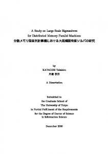
3.4.1 Von Neumann Bottle Neck on the Conventional Computer As described in Section 2.1.1, the current conventional computer has a Von Neumann bottleneck between CPU and main memory. The Processor-DRAM Gap has been becoming larger and larger as shown in Figure 3.15[Fro98].
CPU
“Moore’s Law”
1982 1983 1984 1985 1986 1987 1988 1989 1990 1991 1992 1993 1994 1995 1996 1997 1998 1999 2000
10 1
µProc 60%/yr.
Processor-Memory Performance Gap: (grows 50% / year) DRAM DRAM 7%/yr.
100
1980 1981
Performance
1000
Time
Figure 3.15: Processor DRAM gap[Fro98].
In this situation, the CPU can not display its peak performance as already mentioned in Section 2.1.1. Here, several simulations on a current commercial PC are done to show the Von Neumann bottleneck. Parameters are shown in Table 3.1. The second column values are taken from the PC system Toshiba PortegeTM 620CT. The spec of 620CT is described in Table 3.2. Two programs are executed on the PC. One adds an operand on the main memory with a constant value on a register and stores the result on the main memory (Program A). The other adds two operands on the main memory and stores the result on the main memory (Program B).
26
Chapter 3. Functional Memory Type Parallel Processor: FMPP
Table 3.1: Parameters for a conventional Von Neumann computer. Name Value Synopsis
@�A C@ B D E
10ns.
processor clock cycle
50ns.
main memory access time
64
bus width
8 F 32
bit width to be processed
Table 3.2: Spec of Portege 620CT. CPU
Pentium 100MHz Data Bus Width 64 D-Cache Size
8kB
I-Cache Size
8kB
Main Memory EDO DRAM Size
40MB
Access Time
50ns.
OS
Linux 2.0.32 (a famous UNIX compatible OS for PC/AT)
C Compiler
gcc 2.7.2.3 Option
Program A : Program B :
–O2 (Highly optimized)
GIHJHJGLKNM=O'PRQ5STGIHJHJGLKUG O P)QLVWMYX5Z�[]\ ; GIHJHJGLKNM=O P)Q5S^G_HJHJGLK=G�O'P)Q`VaGIHJHJGLKcbdO'PRQ ;
To execute Program B, the CPU should access the main memory three times: twice to load operands and once to store the result. Similarly, Program A accesses the main memory twice. Thus, to use above parameters, total execution time for these two programs are described by Equation (3.1) and (3.2) respectively.
@CB V @RA S @gB R@ A S [Exec Time of Program B] S 3 e V
[Exec Time of Program A]
S
2e
110ns f 160ns f
(3.1) (3.2)
In Portege 620CT, Program A takes 102ns., while Program B takes 160ns. Note that these are
3.4. Parallel Computation Efficiency on the FMPP
27
average values of huge number of iterations. They are almost equal to the values obtained from Equation (3.1) and (3.2). These results clearly show the Von Neumann bottleneck. The processor has capability to complete addition in 10ns, while each data transfer between the processor and the main memory takes 50ns. It is no use to increase the processor clock frequency on the Von Neumann computer. The execution time is limited by the DRAM access time.
3.4.2 Parallel Computation on the FMPP Figure 3.16 depicts a parallel computing system using the FMPP, which structure is similar to the conventional Von Neumann computer. Some part of the main memory, however, consists of the FMPP. We assume that the FMPP has a capability to perform numerical operations between two words simultaneously in all the PEs. Parameters are defined as follows.
h j@ i
number of clock cycles for numerical operations on the FMPP FMPP clock cycle
D-cache
CPU Register File
Main Memory
(DRAM)
ALU
Instruction Decoder
bus
I-cache
bus
bus
PE
PE
PE
PE
PE
PE
FMPP PE
PE
PE
Instruction
Figure 3.16: A computer system using an FMPP as a part of main memory.
We compare the total execution time on the FMPP system and the Von Neumann system. The operation performs a numerical operation denoted by
k
to a large number of data l
as follows. for P7S 0 to l
m
1
mem[Pnk 3] = mem[Pok 3 V 1] k mem[Pnk 3 V 2]
end
on the memory
28
Chapter 3. Functional Memory Type Parallel Processor: FMPP
1e+09 Vonn Neumann f=1000 f=100 f=10
execution time (nsec)
1e+08 1e+07 1e+06
100000 10000 1000 100 1
10
100
1000 10000 M: Number of data
100000
1e+06
Figure 3.17: Total execution time on the Von-Neumann computer and on the FMPP. The total execution time on the Von Neumann model for a single iteration becomes lperq 3 The FMPP simultaneously performs the same operation for all
t e u@ i .
l
@CB V R@ AJs .
data within the constant time of
l is small. u @ i Figure 3.17 shows the total execution time for l where is assumed to be 50ns as the same value of t the DRAM access time. When S 100 and l S 1000, the FMPP outperforms the Von Neumann The FMPP gets better performance than the Von Neuman computer even when
computer by 32 times. Note that we can neglect the time to prepare data structure on the FMPP. It is becase the same data structure must be prepared on the conventional main memory. Operations on the FMPP are not always superior to the Von Neumann computers, since all the current commercial CPUs have cache memory. Once data come to cache memory, CPU can quickly access the data. If the CPU executes a group of operations for the data size of which is smaller than the cache size, the CPU can access the data directly from the cache memory. It improves the performance of the Von Neuman system. But once a cache misse occurs, the performance is degraded considerably. Several novel cache architectures have been proposed and developed to decrease the cache miss count. Here, we compare the performance between a Neumann computer system with a cache memory and an FMPP system. A series of
v A
operations is performed to a huge number ( l
) of groups of
data, each of which includes the number w of data. Figure 3.18 depicts two systems. We suppose the following conditions. 1. A CPU can access its cache memory in h clock cycles. 2. The size of cache memory xny{z|w
3.4. Parallel Computation Efficiency on the FMPP
CPU
Cache
} ~
29
Main Memory
FMPP
Neumann Computer
Figure 3.18: Von Neumann system with cache memory and FMPP-based system.
3. The CPU can access all the data from its cache memory besides the first load and the last store operations for the main memory. 4. A PE of the FMPP has w words. 5. The FMPP can complete the same operations in v
i S t eJw�eJv A
cycles.
Under the above condition, the CPU can complete the operations in the following period.
@C35 S S
@ q access and store time for DRAM s V @ q Command execution time on the CPU s @CB @�A A 2 ew�e V h e ew�ev (3.3)
On the other hand, the FMPP can complete them
t
times slower than the CPU as follows.
@C3r_ _ S t eJv A e @ui eJw The performance efficiency ¡�¢
¡ ¢ i]i>¤ S S The parameter
l
i£i¥¤
(3.4)
is defined as follows.
C@ 3_= @C3_ _ q 2 e @CB V t h
@CB @�A ¦A s Je l q 2 eJw�e V h Je w�e eJv t eJv A e j@ i e w S e @RA A eJ@uvi A¦s el eJv e
(3.5)
denotes the number of PEs of the FMPP. There are so many parameters in
Equation (3.5). Some actual values are given in Table 3.3. Using these parameters, Equation (3.5) is simplified as follows.
@C3IU A¦s eJl 5 V 2 ev q § i > i ¤ t A S ¡ ¢ S @j3I _I S 5 e ev
5 V 2 ev A 5 eJv
A l e t
(3.6)
30
Chapter 3. Functional Memory Type Parallel Processor: FMPP
¨Table 3.3: Parameters to compare a Neumann Computer system with an FMPP system. Parameter Synopsys
@CB©u@ji h
Value
DRAM/FMPP access time Cache access clock count
5
Figure 3.19 shows the performance efficiency according to lǻ
@�A
t
2
and v
A . As v A
becomes larger,
the performance efficiency asymptotically approaches to 0 f 4 « l ª t . It suggests that an FMPP system t outperforms the Neumann computer by 40 times with l S 1000, S 10. The condition l S 1000 t means that we prepare 1000 PEs, while S 10 means that the required number of clock cycles on the t FMPP can be 10 times bigger than that on the CPU. Note that is the number of clock cycles. The above condition assumes that the clock cycle of the FMPP is 5 times longer than that of the CPU. If the CPU working at 100MHz can complete the operations within 100 clock cycles (1¬ s.), the FMPP
working at 20MHz must complete the same operations within 1000 clock cycles (50¬ s.). The FMPP
is 50 times slower than the CPU. 10000 M/f=1000 M/f=100 M/f=10 M/f=1 M/f=.1
Peformance Efficiency
1000
100
10
1
0.1
0.01 1
10
100
1000
Np (Series of operations)
Figure 3.19: Performance efficiency of an Neumann Computer system / an FMPP system. (M=Number of PEs, f=Number of clock cycles on the FMPP system.)
In the above discussion, we assume conditions as follows. On the FMPP computing system, all the operations are done in the FMPP. On the Neumann computing system, all the data can be obtained from the cache memory besides the first load and the last store operations. It takes 2 clock cycles
3.5. Summary of the Chapter
31
to access the cache. Actually, some part of required data can be directly obtained from registers. It takes a single clock cycle to access the registers. Thus, the comparison may not be accurate. But, even if all the data could be directly retrieved from registers, the FMPP system with a large number of PEs is superior to the Von Neumann computers. The current commercial CPU has various functionalities. Almost all operations such as multiplication can be done in a single clock cycle. In the FMPP, however, a high-performance ALU enlarges the PE area and makes the circuitry complicated. In this paper, we introduced several FMPP implementations which have a capability to complete addition of two words within a single clock cycle. Adders can be implemented with a small number of transistors, while multipliers cost too many transistors. The functions of the FMPP must be defined considering a trade-off between performance and circuit area. In the FMPP-based computing system in Figure 3.16, operations are done both in CPU and FMPP. They have to cooperate to complete a job. Operations must be assigned to the CPU or the FMPP so as to minimize the total operation period.
3.5 Summary of the Chapter In this chapter, we introduce the FMPP architecture. FMPP is a memory-based SIMD shared-bus parallel processor which enjoys the current remarkable progress of semiconductor memory devices. The density of the LSI is doubled every 18 months predicted from the famous Moore’s law. The performance gap between the CPU and the memory device, however, becomes larger and larger. The performance of the current computer system is limited by the bandwidth between the CPU and the memory. The FMPP alleviates the performance gap, since operations can be done inside the memory. As mentioned here, if SIMD operations can be done inside a memory, the performance will improve considerably. The performance of the FMPP is linearly improved according to the number of PEs. The structure of the FMPP similar to that of the memory allows highly dense layout. Communication between PEs, however, is limited. Therefore we must choose the suitable operations for the FMPP. The FMPP can be utilized as two ways. One is as a part of main memory on a conventional Von Neumann computer. The other is used as an application-specific processor. In the former style, an FMPP device can work as both main memory and co-processor. In the latter style, an FMPP device work as a processor independently of the CPU. Here, three FMPP architectures are shown: bit-parallel word-parallel (BPWP), bit-serial wordparallel (BSWP), bit-parallel block-parallel (BPBP). In the BPWP architecture, every PE attached to every bit and word consumes hardware cost. No implementation have been found of the BPWP. The hardware cost of the BSWP architecture is less severe than the BPWP. Lots of associative processors can be found based on the BSWP architecture. A CAM is one of the most popular functional
32
Chapter 3. Functional Memory Type Parallel Processor: FMPP
memory devices. Its word-oriented structure can be regarded as the BSWP FMPP. Extremum search or numerical operations are successfully applied to the CAM. A BSWP FMPP for parallel addition is introduced. It has an ALU for every two words. Here, we mainly focus on the BPBP architecture. It enables operations between two words and operations are done in bit-parallel. We introduce two implementations: the BPBP-FMPP and the FMPP-VQ in the following two chapters. The BPBPFMPP is designed to utilize as a part of main memory. The FMPP-VQ is developed to implement a low-rate image compression system by vector quantization. It can work independently of the CPU. The performance efficiency of the FMPP-based system is also discussed here. The FMPP-based system where a part of main memory is replaced with the FMPP shows better performance than the conventional Von Neumann computing system, if the same operations are applied to huge number of data sets. If we can prepare an FMPP with 1000 PEs which has a capability of numerical operations 50 times slower than the CPU, it can perform series of operations 40 times faster than the Von Neumann system. In the FMPP-based system, we must assign operations to the FMPP or to the processor in order to minimize total execution time.
Chapter 4 An Implementation of the Bit-Parallel Block-Parallel FMPP In this chapter we describe an implementation of the bit-parallel block-parallel FMPP architecture. We have designed and fabricated a prototype LSI[KOT95] BPBP-FMPP based on the BPBP architecture[KTYO93]. The BPBP-FMPP LSI has functionalities of bit-parallel numerical and logical operations on internal two words. Since a CAM cell can execute logical operations on an external data and contents of words, we adopt the structure of a CAM cell as that of a FMPP cell. Using contents of another word as an external data, logical and numerical operations on two words can be performed. We realize bit-parallel addition in combination with logical operations and a carry propagation using a Manchester carry chain[WE85] which propagates the carry in bit-parallel manner. The structure of a CAM cell enables search operations (content addressing) on the FMPP same as that of CAMs. Primary operations on the BPBP-FMPP are summarized as follows.
®
Bit-parallel block-parallel computations such as logical operations, addition, subtraction and multiplication.
®
Search operation.
®
Logical operations on flags.
®
Parallel write operation.
®
Multiple response resolution.
4.1 BPBP-FMPP The BPBP-FMPP can perform parallel numerical operations on internal two words simultaneously on all PEs. It has various functionalities as a RAM, a CAM and a parallel processor. It performs
34
Chapter 4. An Implementation of the BPBP FMPP
addition of two words in a PE in O(1). Multiplication is done in O(¯ ) (¯
stands for the number of
bits of a multiplier). These operations are simultaneously done in every PE. Each PE contains four 32bit words. A single LSI chip contains eight PEs.
4.1.1 Logical Operations on the CAM Cell We utilize the structure of a CAM cell as that of an FMPP cell, since the CAM cell has a possibility of logical operations on an external operand and contents of words. Logical operations on two words can be done on the CAM cell if a content of another word is given as an external operand as shown in Figure 4.1. Suppose that the CAM cell stores
°
and an external data is given through b0 and b1.
The complemental signals ± and ± from b0 and b1 produce ±³²´° , which is within the original CAM
functionality. If one of the bit lines b0 or b1 is dropped to the ground level, logical AND (±µe¦° ) or
logical NOR (±·¶ ° ) operation can be done. b0
b1 q
q
¸0 ¸1 ± ± ± 0 0 ±
¹ º ³ ±³²W° ±»e° ±�¶r°
OL
Figure 4.1: Logical operations on a CAM cell.
4.1.2 Block Diagram Figure 4.2 shows a block diagram of the 1kbit BPBP-FMPP LSI. There are eight PEs, address IO, data IO and other components such as sense amplifiers or control logics. Figure 4.3 depicts the structure of a PE, which comprises a memory block, various flags, a multiple response resolver(MRR) and control logics. The memory block is the essential part of the FMPP, where addition, multiplication and logical operations among two words are performed. The number of words in a single PE is four in this implementation, since at least four words should be required for addition: two words for operands, the other two words for temporary values and the result. They are connected through a shared bus inside the PE called the “local data bus.” The word in a memory block is hereafter called “an operand word.” A memory block comprises four 32bit operand words of FMPP memory cells (w0
F
w3), two 32bit buffers of SRAMs (P, G) and a carry chain. These
SRAMs and the carry chain form an arithmetic logic unit (ALU). The global data bus connect all the memory blocks.
4.1. BPBP-FMPP
35
data bus
address bus
flagin flagout 32
5
data IO data reg.
address reg.
C
C
data mask reg.
address mask reg.
bit0 bit1 RDT
address IO
32 32
chip select
5 global data bus address 32
R
mask
32
sense amp. 32
C
S
Pin
32
PE0 PE1
PE7
C S: sense amp.
R: output register
Pout
C: control logics
Figure 4.2: Block diagram of the BPBP FMPP LSI.
4.1.3 Primary Operations Table 4.1 summarizes primary operations on the BPBP-FMPP. In the memory block, addition, subtraction, multiplication and logical operations are available as a parallel processor. They are explained in detail in Section 4.2. As a CAM, the BPBP-FMPP searches for the operand words matched to a given key data, which functionality is called the search operation. The result from the search operation is stored into master or slave flags. The state of these two flags defines a “selected word.” The multiple response resolver(MRR) resolves a single operand word among the selected words, which is called multiple response resolution. The BPBP-FMPP can perform read/write operations similar to conventional RAMs. In addition to that, the parallel write operation is also available. The FMPP writes data to all the selected words, or to multiple words defined with the address masked by the address mask register located at the address IO. The block flag (BF) prohibits operations of the block on multiplication. The overflow flag(C32)
36
Chapter 4. An Implementation of the BPBP FMPP
memory block master flags
slave flags
m0
s0
m1
s1
m2
s2
m3
s3
w0 Multiple Response Resolver
w1
LU P
LN
w3 OL
local data bus LP
global data bus
w2
matching line
G carry chain
TF
BF
overflow
C32 prohibit operations
PE
memory block
Figure 4.3: Structure of a PE.
stores an overflow value from addition. The temporary flag(TF) temporarily stores a result from the search operation. The operation called the block transfer is used to communicate between blocks (PEs). A block can communicate with its two adjacent blocks. As for interchip communication, however, the BPBPFMPP has data and address buses for both input and output in order to decrease the number of IO pins. Processors on separated LSIs should communicate with each other one by one.
4.1.4 Data Mask and Address Mask Operations Two mask registers, the address mask register (AMR) and the data mask register (DMR) define masks on address and data portions respectively. The mask on the address portion is used to select multiple words. For example, if all bits without LSB are masked, we can choose all the odd or even words by LSB of the address. It is used on the parallel write operation and the search operation. The mask on the data portion is used in three different ways. One is the mask on the search operations. The masked bits becomes the “don’t care” state. These masked bits are always matched. It is used on the multiplication explained in Section 4.2.5. On the search operation, a key data stored in the DR masked by the DMR is compared with the content of a word in the PE. If the address mask is set, only the specified PEs perform the search operation. The other is used on the partial write
4.1. BPBP-FMPP
37
Table 4.1: Primary operations on the BPBP-FMPP. operation
comment
#step
Operations as a parallel processor in a block WPjk W¼¾½ W ¿
logical operations
2
WPgÀ W¼¾½ W ¿
addition/subtraction
ÁÂP )
1 if OW AB8�9;: &"8
resolve the topmost PE whose SF is true.
õ D
2 2
becomes false if there is no true. SF
������EH9@>@>
is the address of the topmost PE.
To write a codebook to codebook words writecode( ������E�9G>"> ,������� )
data write to CW(7 )
2
these operation takes four clock cycles, while the operations where an operand is given from the global data bus such as subtraction does not need any precharge cycle. Figure 5.22 shows the whole procedure to perform the nearest neighbor search. The initflag operation is required on the FMPP-VQ64 because of the design fault. The required number of clock cycles IKJLJNM is described in Equation (5.10). IOJLJNM
÷QP(RTSVUÆùBPXW ñZY$ñ W\[;W)U ] R(^�_V`ØùaPXb�cd`e] ^fU ÷ 24 ó ù 2 g,øúù û log2 ó¿ý�hÆù 8
It takes 470 clock cycles when ó =16 and
(5.10)
ø =12: 416 cycles to compute the absolute distance, 50
clock cycles to obtain the address where the nearest neighbor vector is stored and 4 clock cycles for the other operations. Note that the number of clock cycles does not depend on the number of PEs (i.e., size of a codebook).
5.4. Architecture and Structure
71
1 clock cycle (25MHz)
clock address data output strobe control
perform an operation
code2operand
nop
precharge cycle
actual operation
Figure 5.21: Timing Diagram of the FMPP-VQ.
for i j 0 to 15 # compute absolute distance begin #416cycles=24*16 initflag() |} ~ ~ | code2operand(i ) subtraction(k l ) temp2operand complement temp2operand Σ 10
addinner temp2result end result2operand # 4 m n o p =0b111111111111 o q n r s t u n v =0b000000000000 for i j 11 downto 0 # extract minimum value begin # 48=12*4 m n o p w i x =0 search( o q n r s t u n v m n o p ) mrr( y z ,) o q n r s t u n v w i x =1 if y z = 0 end search( o q n s t u n v )# 2 mrr(, m i { l ) # 2
Figure 5.22: Whole procedure to perform the nearest neighbor search.
72
Chapter 5. FMPP for Vector Quantization: FMPP-VQ
Table 5.4: LSI specifications of the FMPP-VQ4. Process
0.7 m double-metal single-poly CMOS
Die size
26.3mm2
Area for 4 PEs
1.12mm2
# IOs Power dissipation
116 3.8mW @(25MHz,5V)
5.5 Implementations of FMPP-VQ LSIs In this section, two LSI implementations of the FMPP-VQ architecture are introduced. The first LSI contains four PEs called “FMPP-VQ4,” which is for evaluating functionalities of the FMPP-VQ. Almost all functionalities are verified, but we found several faults. Secondly, we have designed and fabricated an LSI with 64 PEs called “FMPP-VQ64.” It can be applied to low bit-rate image compression using vector quantization. It works properly at 25MHz and achieves high performance and low power.
5.5.1 An LSI Including Four PEs and TEGs: FMPP-VQ4 We have implemented an LSI called “FMPP-VQ4” including four PEs and some test circuitries using a 0.7 m double-metal single-poly CMOS process. Four PEs and a 12bit sense amplifier are shown in the chip microphotograph of Figure 5.23. Table 5.4 shows specifications of the LSI. All the primitive control signals to the PEs and sense amplifiers are assigned to the primary input signals of the LSI, which increase the number of IO pins and chip area, while enhancing testability and controllability of the FMPP-VQ. All functionalities to perform the nearest neighbor search work properly at 25MHz, which is the same value obtained from circuit simulations. In the LSI, a 2bit ALU, a sense amplifier and 32bit carry chain are implemented. Unfortunately, they can not work correctly because of a short circuit between the power and ground nodes. In the FMPP-VQ4, several faults are found. The most critical fault is as follows.
At the code2operand operation, 4 MSBs of the operand word becomes unknown state. It is because the local bit lines of these bits are floated on the operation.
In the FMPP-VQ64, these 4 MSBs are connected to the ground node at the code2operand operation.
73
2bit ALU
4PEs
32bit Carry Chain
sense amps.
5.5. Implementations of FMPP-VQ LSIs
Sense Amp.
Figure 5.23: Chip microphotograph of the FMPP-VQ4.
5.5.2 An LSI Including 64 PEs and Control Logics: FMPP-VQ64 We have implemented and fabricated the FMPP-VQ64 LSI using the same 0.7 m CMOS process as that of the FMPP-VQ4. Figure 5.24 shows its detailed block digram. It is controlled by a 5-bit operation code supplied to the IO control logic ICL and the global control logic GCL. The control signals from the GCL to 64 PEs are doubled to decrease the load capacitance and to enhance the performance. Upper and lower 32 PEs are controlled by individual drivers. To equalize the distance from the ICL to every PE, the global data bus is laid out as the shape of an H character. To enhance its testability it has been designed such that all primitive control signals to the PE can be directly given from the IO pins. The number of IO pins is 50 except the primitive control and power supply pins. It is fully functional by the primitive control signals. But the control logics do not work correctly. In the FMPP-VQ4, all the circuitries can be simulated by the transistor level simulator HSPICE\ , while in the FMPP-VQ64 the transistor level simulation is impossible since the number transistors amounts to several hundred thousand. To simulate the whole circuitries of the FMPP-VQ64, we have developed a behavioral HDL description of the PE. Figure 5.25 shows the Verilog-HDL description of the operand word and the carry chain. The whole circuit of the FMPP-VQ64 is simulated in the logic level by the logic simulator Verilog-XL. The fault of the control logics occurs because the HDL description of the PE does not follow their accurate behavior.
74
Chapter 5. FMPP for Vector Quantization: FMPP-VQ
PE#3
#7
operations
Lower 32PEs
PE#8
IO Control Logic
ICL
PE#2
Global Data Bus
GCL
operations
mask
PE#1
CR
Global Control Logic
PE#0
Upper 32PEs
Local Priority Address Encoder
#63
min. distance
ER Address for min. distance.
Global Priority Address Encoder
Figure 5.24: The detailed block diagram of the FMPP-VQ64.
Figure 5.26 shows the chip microphotograph. LSI Specifications of both the FMPP-VQ4 and FMPP-VQ64 are described in Table 5.5. Figure 5.27 shows a measured Shmoo plot of supply voltage versus cycle time. While the recommended supply voltage of the target process is 5.0V, the FMPP-VQ64 LSI works properly at 3.0V/25MHz and at 2.5V/20MHz. The power dissipation of the FMPP-VQ64 is 20mW under the condition of 3.0V/25MHz. Figure 5.28 shows the dynamic current flow of the power-supply pin during an iteration of the absolute distance computation. The operating condition is at 25MHz/5V. The current flow has peaks when operations such as subtraction, complement and addinner are executed.
Table 5.5: LSI specifications of both of the FMPP-VQ4 and FMPP-VQ64. FMPP-VQ4 Process Die size # IOs
0.7 m double-metal single-poly CMOS 26.3mm2
52.6mm2
116
148
Power dissipation
FMPP-VQ64
9.30mW@(20MHz,2.5V) 3.8mW@(25MHz,5V)
20.5mW@(25MHz,3.0V) 128mW@(25MHz,5.0V)
Area of a PE array Area of a PE
2.43mm2 (2 ð 2)
23.5mm2 (8 ð 8)
.28mm2
.37mm2
5.5. Implementations of FMPP-VQ LSIs
75
module operandword (c1_, sum, pp, b0, b1, search, sin, c0_, w0, w1, we); output c1_,sum,pp; inout b0,b1; inout search,sin,c0_,w0,w1,we; reg q,c1; always @(b0,w0,we) #10 case(b0,w0,we) 3’b011: q=0; 3’b111: q=1; endcase not not0(we_,we); and and0(write0,w0,we_); and and1(write1,w1,we_); bufif1 (weak0,weak1) buf0(b0,q,write0); notif1 (weak0,weak1) not1(b1,q,write1); not not2(c0,c0_); xor xor0(sum,q,b0,c0); or or0(pp,x0,x1); not not4(q_,q); not not5(b1_,b1); not not6(b0_,b0); and and2(x0,q,b0_,b1); and and3(x1,q_,b0,b1_); // adder always @(b0,c0,q) begin c1=(b0&&c0)||(b0&&q)||(q&&c0); end not not3(c1_,c1); // search bufif1 bufsearch0(search,sin,pp); endmodule
Figure 5.25: Verilog-HDL description of the operand word and the carry chain.
As described in Section 5.4.5, the FMPP-VQ computes the nearest neighbor search (NNS) in 470 clock cycles. Thus, the FMPP-VQ64 completes the NNS in 18.8 sec at 25MHz. It can perform 53,000 NNSs per second. In order to eliminate unnecessary state changes in the ALU, the inverter in Figure 5.10 is only activated at the numerical operations. To evaluate the effect, power dissipations are measured. Table 5.6 shows the results. Unfortunately, activating the inverter only at the numerical operation increases the power. It may be because the input nodes of the inverter has high probability of high voltage. When the inverter is deactivated and the input node of inverter is high, the output node is floated, which leads short-circuit current in the XNOR gate or the carry chain. To eliminate the short-circuit current, the inverter must be deactivated by both of NMOS and PMOS FETs. But it makes the circuit area larger. Therefore, in the FMPP-VQ64M, which is the modified version of the FMPP-VQ64, the inverter is controlled by a PMOS FET (See Section 5.6.3). Since the input node of the inverter has
76
Chapter 5. FMPP for Vector Quantization: FMPP-VQ
£¤¥
¦ § ¨ ©
¡¢
Figure 5.26: The chip microphotograph of the FMPP-VQ64.
high probability of high voltage, the output node of the inverter has high probability of discharged state causing no short-circuit current in the subsequent circuits when deactivating the inverter. Table 5.6: Comparisons of power dissipation by activating the inverter at the numerical operation and by always activating the inverter. The condition is 5V/25MHz. Activation
at the numerical operations
always
193mW
128mW
Power dissipation
5.5.3 Integration Density of the FMPP-VQ64 Here, we evaluate the integration density of the FMPP-VQ64 compared with a conventional SRAM designed with the same technology. Table 5.7 shows the area of a single PE of the FMPP-VQ64 with the area of the 8kbit SRAM designed with the same 0.7 m process[DAT96]. The 64PEs of the FMPP-VQ64 contains 8kbit codebook words, which area is 9.5 times larger than the conventional SRAM. Looking at Figure 5.5, the global data bus, control lines and address bus occupies about a half of PEs. Without these bus and control lines, the area of the 64PEs is reduced to 10.1mm2 , which is only 4 times larger than the conventional SRAM. The reason why the area becomes twice including
5.5. Implementations of FMPP-VQ LSIs
77
[V] 5 4.5
supply voltage
pass 4 3.5 3
fail
2.5 34
36
38
40
42
44
46
48
50 [ns]
cycle time Figure 5.27: A measured Shmoo plot of supply voltage versus cycle time in the FMPP-VQ64.
these bus and control lines is mainly that the fabricated process has only two metal layers. If the brand-new sub-micron multiple-metal-layer process is available for use, the integration density of the FMPP will increase considerably. Table 5.7: Area for 1 PE of the FMPP-VQ64 and 8kbit SRAM fabricated by the same 0.7 m process. area(mm2 ) 64PEs
23.5
1PE
total
.367
16codebook words+ALU .137 priority address encoder 8kbit SRAM
.02 2.45
5.5.4 Testability of the FMPP-VQ64 To enhance the testability of logic LSIs scan methods have commonly been used. The FMPP-VQ64 adopts the parallel random-access scan methodology[WE93] owing to its memory-based structure. Codebook words can be accessed in the same manner as conventional RAMs. Furthermore, all words and flags in the ALU can be accessed with read/write operations. Figure 5.29 illustrates the address control scheme of the FMPP-VQ64. It has 10-bit address
78
Chapter 5. FMPP for Vector Quantization: FMPP-VQ
0.15
Dynamic Current
0.1
0.05
0
-0.05 code2operand
temp2operand
subtraction
temp2operand
complement
temp2result addinner
Figure 5.28: Dynamic Current flow on the absolute distance computation.
control lines for 1k (16 ª 64) codebook words. Higher 6-bit signals to the higher address decoder (HAD) represent a PE address. Lower 4-bit signals to the lower address decoder (LAD) are used for a codebook-word address in each PE. On SIMD operations, such as subtraction, the input signal «�¬@ ®V®
is set to high. Then all higher decoded addresses become active. All PEs work simultaneously
according to the SIMD control method. On read/write operations, the higher decoded address determines a single PE. In the local control logic (LCL) shown in the bottom left of Figure 5.29, a higher decoded address from the HAD enables the local decoded address ( ¯±°³² ) from the LAD. To append parallel random-access capability to the ALU, the higher decoded address also enables control signals from the global control logic.All words and flags in the ALU can be accessed through read/write operations, which improves the testability of the FMPP-VQ64 considerably. The number of signals controlled by a higher decoded address is only 10 in the ALU. The hardware overhead is very small. Note that the flags are connected to the local data bus as shown in Figure 5.4 in order to be read or written directly through the bus.
5.6 Modified Version of the FMPP-VQ: FMPP-VQ64M The FMPP-VQ64 achieves both of high performance and low power. But it has some drawbacks to compute the NNS as follows. Eight operations are required to compute the absolute distance of a single dimension, as already shown in Figure 5.22. Half of these 8 operations transfer a value from one word to another such as temp2operand. These transfer operations decrease the throughput
5.6. Modified Version of the FMPP-VQ: FMPP-VQ64M
79
4 address 64 8
higher decoded address(HDA)
codebook words
rcall
LCL
6
Higher Address Decoder(HAD)
PE#0 LDA[0] LDA[1]
PE#1
ALU CW[0] CW[1]
PE#7
SF OF
PE#8
HDA LDA[15]
CW[15] PE#56
GCL
ALU
Local Control Logic(LCL)
PE#63
PE array Global Control Logic(GCL)
16 LDA[0:15]
lower address decoder(LAD)
Figure 5.29: Parallel random-access capability to the ALU.
and increase the power consumption. The number of operations can be reduced if operation results are directly written to the OW . The optimal transistor-sizing may reduce the short-circuit power dissipation. In this section, a modified-version of the FMPP-VQ64 is described, which is called “FMPP-VQ64M.” The structure of the FMPP-VQ64M is similar to the FMPP-VQ64. But it can perform 91,000 NNSs per second which is almost two times faster than the FMPP-VQ64. It integrates a highlyfunctional control logic to manage the nearest neighbor search.
5.6.1 Structure of a PE Figure 5.30 compares two PE structures of FMPP-VQ64 and FMPP-VQ64M. Codebook words are 16 words of eight-bit conventional SRAM cells, which store a 16-dimensional code vector. The ALU computes the absolute distance. The operand word receives data from the local data bus and performs logical operations. In the FMPP-VQ64, operation results from the carry chain or the operand word are temporarily written to the temporary word. To reuse the value stored in the temporary word, it must be transferred to the operand word, which always consumes an operation. To remove such drawbacks, the ALU of the FMPP-VQ64M does not have the temporary word. Operation results can directly be written to the operand word. It can compute the absolute distance for an element ´¶µ of ´ · in four steps, while the FMPP-VQ64 takes eight steps.
Chapter 5. FMPP for Vector Quantization: FMPP-VQ
lb0
lb0
Codebook Words x16
lb1
CW(0)
Local Bit Line
CW(0)
Local Bit Line
80
Codebook Words x16
CW(15)
CW(15)
8bit
8bit
12bit
12bit
Result Word RW
Result Word RW
Operand Word OW &
Operand Word OW &
SF
CR
search lines
search lines
Carry Chain
C0
Carry Chain
ALU
OF
ALU +
+ Temporary Word TW
(a)
(b)
Figure 5.30: PE structures of the FMPP-VQ64(a) and the FMPP-VQ64M(b).
5.6.2 Absolute Distance Computation In the FMPP-VQ64M, the absolute distance is computed element by element according to Equation (5.11).
¸eÅ ¹º 1 ¼ ÁÂÂ
¹º
¸
º�½¿¾ ¼
» 0
´
ÂÂ Â º Ã
¼?À µ
ÂÂ
ÂÂ ÂÄ
º ½¿¾
º ¾
½
¾
¼@Æ
µ µ¸ ´ ´ ¸ » 0 º�½B¾ º ¾ ½ ¸eÅ 1 Ë ¹º ¼ ¼ Æ Ç ´ µ Ê µ¸ » 0
Ç
µ ¸ÉÈ
´ ¸"Ê
¾ Ç
´ ¸HÌ ¾
It requires a conditional operation according to the results of
(5.11) µ ¸ÉÍ
´ ¸ Ê
½ µ
´-µ
, which is enabled by the
overflow flag OF. Three operations as shown below compute the absolute distance. ¾
Operation 1 Compute
½ µ¸
´ ¸ ¾
Condition 1
ÎÇ
½ µ¸ ¾
Operation 2 Condition 2
ÎÇ
¾ È
´ ¸
0 Ê�Ï
µ¸
Accumulate
½ µ¸
½
¾ ´ ¸ÐÍ
0 Ê�Ï
Accumulate
´ ¸
to
½ µ¸
´ ¸
to
º�½¿¾
¸eÅ ¹º 1 ¼ » ¸ Å 0 e ¹º 1 ¼ » 0
º ¼
´
.
µ
´
º�½¿¾ µ
º ¼
.
5.6. Modified Version of the FMPP-VQ: FMPP-VQ64M
Operation 3
¾
½
Condition 1
Î Ç ¾ µ¸ ½
Condition 2
Î Ç
È
0 Ê�Ï
Transfer the original value to the RW .
´ ¸ÐÍ
0 Ê�Ï
Transfer the inversed value to the RW .
´ ¸
µ¸
81
These operations are performed in 4 steps as below. ¾
¾
Step1: [code2operand(Ñ )] The Ñ th element of Step2:¾
· µ
,
[subtraction( ´ ¸ )] The Ñ th element of ´ · , ´ ½
¸
µ¸
´-µ
µ¸
is sent to the OW.
is broadcast to all PEs. Then, the subtraction,
is done. The result is stored in the OW. The overflow value is stored in the OF. ¾
½
Ç
´ ¸ ÊÒÈ
µ¸ ¾
Step3: [addinner]
0
½
Ç
´ ¸ Ê
µ¸
Ç
Step4: [temp2result] Ç
¾
½ ¸ ¾ µ ½
µ¸
Í
0
´ ¸@ÊÒÈ ´ ¸ Ê
» 0 ¸eÅ ¹º 1 ¼ » 0
0 Í
º�½B¾
¸ÓÅ ¹º 1 ¼
0
´
º µ
º�½¿¾ ´
¼GÆÕÔ×ÖÙØ
ÔÒÖ
¼"ÆÕÔ�ÖÙØ
Ô�Ö
º µ
Ô�ÖÚØ
Û¶Ö
Ô�ÖÙØ
Û¶Ö
. .
At Step1, an element of code vectors is tranfer to the operand word. There exists no useless transfer operation between the other operations. At Step2, ´ ¾ ½ µ¸
subtraction
´ ¸
¸
is given through the local data bus and ¾ ½
is done. The overflow value º�½¿¾ is º stored to the OF . If º
1. At Step 3 and 4, the summation Ü
¸eÅ 1 ¼ » 0 ´
µ
¼
is accumulated to
¼
È
µ ¸ ½¿¾ ´ ¸
´ ¸
µ¸
¼
0, the OF becomes
. The value º�½BOF ¾ º º of the
controls the operations at these two steps. The final value stored in the RW becomes
¸
Ü
¼ » 0 ´
µ
¼
at the both conditions. Figure 5.31 depicts the data flow to compute Equation (5.11) (in page 80). It shows conditions ¾ two ½ according to the results of the subtraction in Step2. The upper condition¾ is where the lower one is the opposite state. In Step1, code2operand transfers Step2 all PEs receive an element ´
¸
µ¸
µ¸
´ ¸
È
0 and
from CW(Ñ ) to OW . In
of an input vector ´ · . In Step 2’, the subtraction between ´
¸
and
the OW is performed and the results are written to the OW and the OF . In Step 3 addition between the RW and the OW is done and the result is written to the OW . The value from the RW to the local data bus is changed according to the OF . In Step 4, the value in the OW is moved to the RW , which ½¿ ¾ º ¸
becomes Ü
¼ » 0 ´ ¸
µ¸
¼
.
5.6.3 Detailed Structure of the ALU Figure 5.32 shows a detailed schematic diagram of two-bit slice of the ALU. Figure 5.33 shows a detailed schematic diagram of the operand word. When an operation between the OW and an operand from the local bit lines is done, the result is written to the OW itself. To write back the operation
82
Chapter 5. FMPP for Vector Quantization: FMPP-VQ
�� ä è é ê ëä
1
0
æç
æ
OW
local data bus
binary
ï ðñ ôõ ö÷ ø
RW
1
0
ùú
1ò ó ÷ û ü ýþ ÷ 1ÿ
OW
� ��
decimal
0110 (6)
0110 (6)
1000 (8)
1000 (8)
1000 (8)
0110 (6)
binary
1
ù
’
decimal
0011 (3)
0011 (3)
0011
(3)
0101 (5)
0101 (5)
0101
(5)
0011
(3)
0001 (1) 1
3
(3)
0101
(5)
1110 (-2) 0
3
1000 0
(5) 0110 0
’
addinner
0110 (6)
(add -5 and OW) 0011
0011 (3)
addinner
0110 (6) 1000 (8)
0110 (6)
1
(add -5 and OW)
OF
2
2 subtraction(5)
0110 (6)
OF
CW(j)
0110 (5)
1 code2operand(j)
global data bus
local data bus
áâ ãä å
RW
íì î
Ý Þ ßà
CW(j)
Step initial state
0110 (5)
1
4 operand2result
0110 (6)
0110 (6)
1000 (8)
1001 (9)
0001 (1) 1
1001 (9) 1
1001 (9) 1
(add -5 and OW)
(add -5 and OW)
(add -5 and OW)
1000 (8)
0011
(3)
0101
(5)
1110 (-2) 0
1000
0110 (5)
0011
(3)
0011
(3)
0101
(5)
0111
(7)
1000
(7) 0
1000
(7) 0
Figure 5.31: A single dimension slice of the absolute distance computation in FMPP-VQ64M.
result to the OW safely, two CMOS switches Sw0 and Sw1 are cut off. The gate capacitance of nodes T and
�
holds the value stored in the OW .
In the result word RW (See Figure 5.35), W0 and W1 are controlled by the value of the
�� Ô
, which
enables read and write operations of the inversed value required at Step3, 4. The controlled inverter in Figure 5.34 decreases power consumption considerbly. The control signal
�
����� �� is activated on
the numerical operation. As already written in Section 5.5.2, the input node of the inverter has a high probability of high voltage. Once its output node is discharged, it can not be re-charged unless � � �����
� is activated. THus, the XNOR gate and the carry chain dissipate power at numerical operations. Table 5.8 compares the specifications of the PEs of FMPP-VQ64 and FMPP-VQ64M. The number of transistors in the FMPP-VQ64M is decreased to 86% compared to that in the FMPP-VQ64, while the area of PE is almost same. It it mainly because the number of vertical signals in the ALU increases.
5.6. Modified Version of the FMPP-VQ: FMPP-VQ64M
83
local data bus
lb0
lb1
lb0
lb1
Result Word
W0 W0 WE
WE W1 W1 W1 WE WE2
Operand Word
W0
CALC WE2 WE
search lines sum0 control
sum2
G P
XNOR
C0
C2
Carry Chain
INV
Figure 5.32: Two-bit slice of the ALU.
The total number of transistors in the PE is increased, since the local control logic to manage W0 and W1 in the RW becomes complecated. The number of clock cycles to compute the absolute distance, however, is decreased to 53% of the FMPP-VQ64.
5.6.4 A Highly-Functional Control Logic The FMPP-VQ64 has a primitive control logic which translates a specified 5-bit control code to primary input signals of the PE array. In the FMPP-VQ64M, a highly-functional control logic is implemented. It receives a start signal and automatically performs the nearest neighbor search. It is called the auto-execution mode. To enhance its testability, all primary input signals are directly controlled in the primary control mode. In order to observe some temporary values which are on the way of operations, a HALT signal is given to the control logic. There exist two modes in the auto exectution mode. One is the normal operation mode and the other is the fast operation mode. In the normal operation mode, all operations are done in a single cycle. On the other hand, in the fast
84
Chapter 5. FMPP for Vector Quantization: FMPP-VQ
lb0
lb1 SRAM
WE2
WE
W0
W1
Pt0
B
Pt1
T
Pt2
Sw0
Pt3
T
Sw1
B
CALC
Control IN
OUT
WE
WE2
Figure 5.34: Inverter controlled by a PMOS FET. IN
P
G
Figure 5.33: Structure of the operand word. lb1
lb0
Auto Execution Mode HALT
W0 W0 WE
Normal Operation Mode
Halt mode Return
Tr0
Tr1 SELECT Return
Tr2
Tr3 Fast Operation Mode
WE
Primary Control Mode
W1 W1
Figure 5.36: The flow of mode changes in the FMPP-VQ64M.
Figure 5.35: Structure of the result word.
opearation mode, numerical operations are done in two cycles. In Figure 5.31, numerical operations such as subtraction and addinner can be divided two phases. The second phase is denoted by a single quotation mark. At the first phase, an operand is given to the operand word. At the second phase, the result is written to the operand word. The numerical operations take twice as long as the other non-numerical operations. If the numerical operations are done in two cycles, the clock cycle can be shortened. Thus, the whole operation can be done faster. The detailed simulation results and performance estimation are given afterwards.
5.6.5 Specification and Implementation Equation (5.12) and (5.13) show the number of clock cycles to compute the NNS in the normal operation mode and the fast operation mode respectively.
�����������
º À
14
�
16
Æ
50
À
274
(5.12)
5.6. Modified Version of the FMPP-VQ: FMPP-VQ64M
85
Table 5.8: Comparison of areas and performance for the FMPP-VQ64 and the FMPP-VQ64M. FMPP-VQ64 FMPP-VQ64M # of Tr. per bit in the ALU
45
39
Area of a PE
.241mm2
.238mm2
# Trs of a PE
1524
1534
26
14
# of clock cycles to compute the absolute distance of a single dimension
� �!�#"%$ À
18
�
16
Æ
50
À
338
(5.13)
We estimate that the FMPP-VQ64M works at 25MHz (40ns.) at the normal operation mode. The numerical operations on the FMPP are 1.5 times slower than the other operations. The operation speed can be 1.5 times faster in the fast operation mode, resulting 37.5MHz clock frequency. Thus, the FMPP-VQ64M performs 91,000 NNSs per second at the normal operation mode, while it performs 111,000 NNSs per second at the fast operation mode. Table 5.9 lists power consumption values of a PE from circuit simulations, which shows the effect of two optimizations compared with the FMPP-VQ64. First, the transistor size is optimized to reduce the short-circuit current, which decreases the power by 6%. The controlled inverter decreases the power by 23%. Table 5.10 shows the dissipated power in each part of the PE. It proves that the carry chain dissipates half of the total power. The FMPP-VQ64 activates the carry chain three times in a single dimensional absolute distance computation, while the FMPP-VQ64M activates it twice. Table 5.9: Power consumption of the FMPP-VQ64M from circuit simulations of a PE at 25MHz 5.0V. Optimization Method FMPP-VQ64
Power 3.03mW
before optimizing Tr. size
2.01mW
after optimization
1.86mW
activate INV at operations
1.45mW
FMPP-VQ64M
The power consumption expected from that of the FMPP-VQ64 is shown in Table 5.11. The power consumption of the FMPP-VQ64M decreases by half, while the number of operations for the nearest neighbor search becomes twice of the FMPP-VQ64’s. Thus, its total energy consumption becomes 1/4 compared with the FMPP-VQ64.
86
Chapter 5. FMPP for Vector Quantization: FMPP-VQ
Table 5.10: Power dissipation map for all & the components in a PE.
Table 5.11: The power consumption of the FMPPVQ64M expected from the measured results of the FMPP-VQ64.
whole PE
1.45mW
100%
Carry Chain
0.82mW
56%
Operand Word 0.32mW
22%
Clock Freq.
28.5MHz
25MHz
20MHz
XNOR
0.07mW
5%
Supply Volt.
5.0V
3.0V
2.5V
Result Word
0.06mW
4%
Power(mW)
65
9.9
4.5
Others
0.11mW
11%
The FMPP-VQ64M is designed using the same double-metal single-poly 0.7' m CMOS process as that of the FMPP-VQ64. The layout pattern of the PE is shown in Figure 5.37. At the first stage when we start to design the FMPP-VQ64M, we expected that the area for a PE would be smaller than that of the FMPP-VQ64, since the PE of the FMPP-VQ64M has no temporary word. But the area of the PE becomes almost the same. Table 5.12 summarizes the number of transistors and area for each part in the PEs. The areas for the operand word and the result word in the FMPP-VQ64M becomes larger than those in the FMPP-VQ64. Table 5.12: Areas for PEs of the FMPP-VQ64 and FMPP-VQ64M. FMPP-VQ64M
FMPP-VQ64
# of Tr/bit.
Area/bit
# of Tr/bit.
Area/bit
Codebook Word
6
433 ( 4' m2
6
433 ( 4' m2
Result Word
10
Operand Word
17
Carry Chain
11
XNOR
6
571 ( 2' m2
6
Temporary Word
N/A
N/A
10
Others
2
168 ( 0' m2
2
One bit slice of a PE (for 8LSBs)
142
11205' m2
148
11203' m2
Total (12bit) of a PE
1534
0.214mm2
1522
0.208mm2
840 ( 0' m2 1714' m2
695 ( 5' m2
8 15 11
710 ( 1' m2 977 ( 4' m2 695 ( 5' m2 571 ( 2' m2 930 ( 7' m2 168 ( 0' m2
Figure 5.38 shows the chip micrograph. The die size of the FMPP-VQ64M is 52.7mm2 . Table 5.13 compares the areas of FMPP-VQ64 and FMPP-VQ64M. FMPP-VQ64M actually integrates more complex control logics than that of the FMPP-VQ64. Table 5.14 summarizes the number of implemented standard cells in each control logic. These areas are almost same with both implemen-
5.6. Modified Version of the FMPP-VQ: FMPP-VQ64M
87
tations. It is because the strategies of place and route are changed. The FMPP-VQ64 is placed and routed from the bottom to the top level. Each component such as the PE array or control logics are placed and routed respectively. Then the top level layout is created using these macro blocks. In the FMPP-VQ64M, however, full-custom components such as the PE array or sense amplifiers are placed as macro blocks, but the other random-logic cells in the control logics are placed and routed in the top level with these macro blocks. This strategy decreases the area of the control logic. The FMPP-VQ64M is now under test. Test results will be shown in later.
Address Bus
Misc. Control Lines
Flags, etc.
Codebook Words
64PEs
Highly functional control logic
Global Data Bus
ALU
Figure 5.37: Layout of a PE.
Figure 5.38: Chip micrograph of the FMPPVQ64M.
Table 5.13: The areas for FMPP-VQ64 and FMPP-VQ64M. FMPP-VQ64M Die size (Including I/O PADS) 6 ( 63
52.64mm2
Core size (Without I/O PADS)
40.98mm2
64 PEs
� 7 ( 94mm2 5 ( 78 � 7 ( 09mm2 3 ( 70 � 6 ( 35mm2
23.50mm2
FMPP-VQ64 6 ( 60
� 7 ( 86mm2 5 ( 75 � 7 ( 01mm2 3 ( 52 � 6 ( 24mm2
51.84mm2 40.30mm2 21.97mm2
88
Chapter 5. FMPP for Vector Quantization: FMPP-VQ
Table 5.14: Number of standard cells for control logics. Logics
FMPP-VQ64M
FMPP-VQ64
D-FF
313
45
Other sequential logic cells
1956
548
Total
2269
593
5.7 Comparison with Other Implementations In this section, several comparisons between the FMPP-VQ with the other implementations are given.
5.7.1 Comparison with the Other Vector Quantizer. Here, the FMPP-VQ is compared with the other vector quantizers. Parameters for vector quantization are given again:
� *
)
dimension of vectors number of code vectors bit width of vectors
The compared points are as follows. Codebook optimization It is to hard to obtain a generalized codebook which can be applied to any type of images. It should be optimized for every frame of image. Thus, a codebook has to be updated in real-time. Accuracy of the nearest vector If the vector from the NNS is a suboptimal one, the distance becomes larger, which decreases the quality of a reconstructed image. IO bandwidth A large IO bandwidth enlarges the area and causes problems to mount the LSI on a circuit board. Power Consumption Power consumption should be minimized for mobile telecommunication. There are two algorithms to search the nearest neighbor vector. The tree-searched VQ (TSVQ) has less codebook search complexity in proportion to the logarithmic order of the size of a codebook than the full-searched VQ (FSVQ) adopted in the FMPP-VQ. But the size of memory to store a codebook becomes large. As for codebook optimization, the TSVQ has a major drawback that the
5.7. Comparison with Other Implementations
89
codebook cannot be optimized in real time, since it requires huge computation complexity to generate the tree-structured codebook. Fang et al. proposed a systolic binary tree-searched vector quantizer[FCS+ 94]. Its block diagram is drawn in Figure 5.39. In conventional TSVQ implementations, the total size of a codebook reaches O( Ü-,�.
� .0/21
). The value 1 means the number of levels and
� .
is the number of code vectors in each
sub-codebook. They reduce the size of a sub-codebook at each level into two, which results 2 Ç4365 1 Ê
code vectors in all the sub-codebook. The index of the nearest code vector in a sub-codebook is computed using the MSE as follows.
7 . 5 7 . 1 0 8
;9 < : 5 = :. 1 9 2 5 9�< : 5 = :. 0 9 2 8 = :. 12 5 = :. 02 5?> = :. 1 5 = :. 0 @ < : 7 . 5 7 . 0 if 1 0 A B 30CED
No.C-475, p.197 (1995). 11.
� B ��Pd4 ÁeROS ¨!T a�b�cs , q t uvlw , ¾ y zq|h} “ :ÏO�lÅзÇÒLÀÓ $ « ¨ «jÿ�h¦f§(W!X ©jY�[k\ ± _6¸f§j¹sº»j¼l½ � ÍsÎLf!g * h�i ”, 1995 F ¤s Ósñ�^ »f¼
12.
13.
14.
,
No.C-476, p.198 (1995).
l�m;I�n , o!p q�r , sVt�u(v w “ x�y{z9��|$}$~Oy:4;��|!�6O�
��*(��|6$~ y (;( ”, 1996 F���! ���