AND AIR-CONDITIONING (HVAC) SYSTEM” submitted by Mr. SATHYAM .....
MLP-Emotional BP, FLANN-BP and Neuro-Fuzzy (ANFIS) using MATLAB
R2008a. And ..... In 1911, Mr. Carrier, who is called the ―father of air
conditioning,‖.
A STUDY ON NEURAL NETWORK BASED SYSTEM IDENTIFICATION WITH APPLICATION TO HEATING, VENTILATING AND AIR CONDITIONING (HVAC) SYSTEM
A THESIS SUBMITTED IN PARTIAL FULFILLMENT OF THE REQUIREMENTS FOR THE DEGREE OF
Master of Technology In ELECTRONIC SYSTEMS AND COMMUNICATIONS
By
SATH YAM BONALA ROLL. NO: 207EE107
----------------------------------------------------------------------------------------------------------------
Department of Electrical Engineering National Institute of Technology, Rourkela May, 2009
A STUDY ON NEURAL NETWORK BASED SYSTEM IDENTIFICATION WITH APPLICATION TO HEATING, VENTILATING AND AIR CONDITIONING (HVAC) SYSTEM
A THESIS SUBMITTED IN PARTIAL FULFILLMENT OF THE REQUIREMENTS FOR THE DEGREE OF
Master of Technology In ELECTRONIC SYSTEMS AND COMMUNICATIONS
By SATHYAM BONALA
ROLL. NO: 207EE107 Under the Guidance of
Prof. Bidyadhar Subudhi
----------------------------------------------------------------------------------------------------------------
Department of Electrical Engineering National Institute of Technology, Rourkela May, 2009
National Institute Of Technology Rourkela-769008, Orissa
CERTIFICATE This is to certify that the thesis entitled, ―A STUDY ON NEURAL NETWORK BASED SYSTEM IDENTIFICATION WITH APPLICATION TO HEATING, VENTILATING AND AIR-CONDITIONING (HVAC) SYSTEM” submitted by Mr. SATHYAM BONALA in partial fulfillment of the requirements for the award of Master of Technology Degree in Electrical Engineering with specialization in “ELECTRONIC SYSTEMS AND COMMUNICATIONS” at the National Institute of Technology, Rourkela is an authentic work carried out by him under my supervision and guidance.
To the best of my knowledge, the matter embodied in the thesis has not been submitted to any other University / Institute for the award of any Degree or Diploma.
Date:
PROF. BIDYADHAR SUBUDHI SUPERVISOR
ACKNOWLEDGEMENTS This project is by far the most significant accomplishment in my life and it would be impossible without people who supported me and believed in me.
I would like to extend my gratitude and my sincere thanks to my honorable, esteemed supervisor Prof. Bidyadhar Subudhi, Head, Department of Electrical Engineering. He is not only a great lecturer with deep vision but also most importantly a kind person. I sincerely thank for his exemplary guidance and encouragement. His trust and support inspired me in the most important moments of making right decisions and I am glad to work under his supervision.
I want to thank all my teachers Prof. J.K. Satapathy, Prof. S. Das, Prof. D. Patra, Mrs. K.R. Subhashini, Mr. S. Mohanthy and Mr. Debashish Jena for providing a solid background for my studies. They have been great sources of inspiration to me and I thank them from the bottom of my heart.
I would like to thank all my friends and especially my classmates for all the thoughtful and mind stimulating discussions we had, which prompted us to think beyond the obvious. I’ve enjoyed their companionship so much during my stay at NIT, Rourkela.
I would like to thank all those who made my stay in Rourkela an unforgettable and rewarding experience.
Last but not least I would like to thank my parents, who taught me the value of hard work by their own example. They rendered me enormous support being apart during the whole tenure of my stay in NIT Rourkela.
SATHYAM BONALA
CONTENTS Page No. Abstract List of Figures Abbreviations Chapter 1 Introduction
i ii iii 1
1.1. Introduction
2
1.2. Background study
3
1.3. Motivation
8
1.4. Literature Review
9
1.5. Problem Formulation
10
1.6. Implementation Approaches
11
1.7. Contribution of the Thesis
11
1.8. Thesis Layout
11
Chapter 2 HVAC System Model
13
2.1. Introduction
14
2.2. Working of an HVAC System
14
2.3. HVAC system model
16
2.4. Simulation Results
18
2.5. Heating and cooling.
20
2.6. Heating system.
24
2.7. Ventilating system.
24
2.8. Air conditioning system
25
Chapter 3 System Identification Using Artificial Neural Networks
27
3.1. Introduction
28
3.2. Neuron Structure
29
3.3. Multilayer Perceptron
32
3.4. Simulation Results
35
3.5. Functional Link ANN
37
3.6. Simulation Results
39
Chapter 4 Modified Back propagation and Back propagation algorithms
42
4.1. Introduction
43
4.2. Emotional Back propagation Learning Algorithm.
46
4.2.1 Input-layer neurons.
46
4.2.2 Hidden-layer neurons.
46
4.2.3 Output-layer neurons.
48
4.2.4 The emotional Back propagation parameters
49
4.3. Back propagation weight updation Rule.
51
4.4. Simulation Results
57
4.5. Comparison of Results
59
4.6. Performance of different techniques
60
Chapter 5 Adaptive Neuro-fuzzy inference system
61
5.1 Introduction
62
5.2. Fuzzy If-Then Rules and Fuzzy Inference Systems
62
5.3. ANFIS: Adaptive Network-Based Fuzzy-inference System
65
5.4. ANFIS Learning Algorithm
70
5.5. Simulation Results
71
Chapter 6 Conclusions and Suggestions for future work
73
6.1 Conclusions
74
6.2 Suggestions for Future Work
74
References
75
ABSTRACT Recent efforts to incorporate aspects of artificial intelligence into the design and operation of automatic control systems have focused attention on techniques such as fuzzy logic, artificial neural networks, and expert systems. Although LMS algorithm has been considered to be a popular method of system identification but it has been seen in many situations that accurate system identification is not achieved by employing this technique. On the other hand, artificial neural network (ANN) has been chosen as a suitable alternative approach to nonlinear system identification due to its good function approximation capabilities i.e. ANNs are capable of generating complex mapping between input and output spaces. Thus, ANNs can be employed for modeling of complex dynamical systems with reasonable degree of accuracy. The use of computers for direct digital control highlights the recent trend toward more effective and efficient heating, ventilating, and air-conditioning (HVAC) control methodologies. The HVAC field has stressed the importance of self learning in building control systems and has encouraged further studies in the integration of optimal control and other advanced techniques into the formulation of such systems. In this thesis we describe the functional link artificial neural network (FLANN), Multi-Layer Perceptron (MLP) with Back propagation (BP) and MLP with modified BP called the emotional BP and Neuro fuzzy approaches for the HVAC System Identification. The thesis describes different architectures together with learning algorithms to build neural network based nonlinear system identification schemes such as Multi-Layer Perceptron (MLP) neural network, Functional Link Artificial Neural Network (FLANN) and ANFIS structures. In the case of MLP used as an identifier, different structures with regard to hidden layer selection and nodes in each layer have been considered. It may be noted that difficulty lies in choosing the number of hidden layers for achieving a correct topology of MLP neural identifier. To overcome this, in the FLANN identifier hidden layers are not required whereas the input is expanded by using trigonometric polynomials i.e. with cos(nπu) and sin(nπu), for n=0,1,2,…. The above ANN structures MLP, FLANN and Neuro-fuzzy (ANFIS Model) have been extensively studied.
i
LIST OF FIGURES Figure No.
Page No.
1.1 Block Diagram of System Identification
4
1.2
Type of adaptations
6
1.3
Direct Modeling
6
1.4
Inverse Modeling
8
1.5 Implementation of System Identification Technique
10
2.1
Air flow diagram
15
2.2
HVAC System model
16
3.1
Neuron Structure
29
3.2
Structure of Multilayer Perceptron
32
3.3
Neural Network with Back Propagation Algorithm
33
3.8
Structure of FLANN
38
4.1
Input/output configuration of input layer neuron
45
4.2
Input/output configuration of hidden layer neuron
46
4.3
Input/output configuration of output layer neuron
48
4.4
Multilayer perceptron
51
4.5
Notation for back propagation rule
52
5.1
Fuzzy inference system
62
5.2 Fuzzy if-then rules and fuzzy reasoning mechanisms
64
5.3 (a) Type-3 fuzzy reasoning
66
5.3(b) Type-3 ANFIS (Basic structure of ANFIS)
66
5.4(a) Type-1 fuzzy reasoning
67
5.4 (b) Type-1 ANFIS
68
5.5(a) 2 Input type-3 ANFIS with 9 rules
69
5.5(b) Fuzzy Subspaces
69
ii
ABBREVIATIONS USED ANN
Artificial Neural Network
MLP
Multilayer Perceptron
FLANN
Functional Link Artificial Neural Network
BP
Back Propagation
FIR
Finite Impulse Response
IIR
Infinite Impulse Response
MSE
Mean Square error
HVAC
Heating ventilating and Air conditioning
IAQ
Indoor air quality
ICU
Intensive air uit
CFM
Cubic feet for minute
BPA
Back propagation algorithm
EmBP
Emotional Back propagation
RTU
Roof top unit
CER
Clean Environment Rooms
ISI
Inter Symbol Interference
VOC
Volatile organic compounds
ANFIS
Adaptive Neuro-fuzzy inference system
iii
CHAPTER 1 INTRODUCTION
1.1 INTRODUCTION System Identification is an essential requirement in areas such as control, communication, power system and instrumentation for obtaining a model of a system (plant) of interest or a new system to be developed. For the purpose of development of control law, analysis fault diagnosis, etc. Major advances have been made in adaptive identification and control, in past few decades for identifying linear time-invariant plants with unknown parameters. The choice of the identifier structure is based on well established results in linear systems theory. Stable adaptive laws for the adjustment of parameters in these which assures the global stability of the relevant overall systems are also based on properties of linear systems as well as stability results that are well known for such systems [1]. In this thesis, the major interest is in the identification of nonlinear dynamic systems using Neural Networks. The climatisation of rooms in buildings can be quite a complex control problem if high degrees of comfort and energy saving are required. There are many factors influencing an environment: humidity, outdoor temperature, solar radiation, neighbouring rooms, people presence, furniture in the room, heat sources (as computers), windows, heaters, coolers etc. All these factors have a complex interaction with the comfort and the energy demand. From the automation point of view, the objective of modeling a building is not to precisely calculate the temperature in every point of a room, but to have information that can lead to a successful controller design. This means that the distributed, continuous, and eventually non-linear process should, with sufficient precision, be described by a lumped LTI parameters model. If the room is architecturally well designed and the actuators well placed, comfort and energy-saving can be obtained. A predictive HVAC controller can potentially obtain the best compromise between comfort and energy saving. The scheduled room occupation can be prepared with the just needed in-advance acclimatization, a quite unique characteristic of predictive controllers. The nonlinear functional mapping properties of neural networks are central to their use in identification and control. Although a number of key theoretical problems remain, results pertaining to the approximation capabilities of neural networks demonstrate that they have great promise in the modeling of nonlinear systems. An important question in system identification is whether a system under study can be adequately represented within a given model structure. In the absence of such concrete theoretical results for neural networks, it is
2
usually assumed that the system under consideration belongs to the class of systems that the chosen network is able to represent.
1.2 BACKGROUND STUDY The area of system identification is one of the most important areas in engineering because most of the dynamical system behavior can be obtained exploiting system identification techniques. For identifying an unknown dynamic systems two things are important i.e. model structure and then parameters. Adaptive Modeling and System Identification are prerequisite before going to design a controller for an on-line plant, say for a scenario an on-line plant requires a controller for improving its performance. The controller cannot be operated on the on-line plant as it may disturb the entire production which may be cost effective, so a model is required which represents the on-line plant. Here comes the concept of modeling a plant. If there is Adaptability in modeling there is more chance of controlling the model on-line thus Adaptive modeling of a plant is done. System identification concerns with the determination of a system, on the basis of input output data samples. The identification task is to determine a suitable estimate of finite dimensional parameters which completely characterize the plant. The selection of the estimate is based on comparison between the actual output sample and a predicted value on the basis of input data up to that instant. An adaptive automaton is a system whose structure is alterable or adjustable in such a way that its behavior or performance improves through contact with its environment. Depending upon input-output relation, the identification of systems can have two groups
A. Static System Identification In this type of identification the output at any instant depends upon the input at that instant. These systems are described by the algebraic equations. The system is essentially a memory less one and mathematically it is represented as y(n) = f [x(n)] where y(n) is the output at the nth instant corresponding to the input x(n).
B. Dynamic System Identification In this type of identification the output at any instant depends upon the input at that instant as well as the past inputs and outputs. Dynamic systems are described by the difference or
3
differential equations. These systems have memory to store past values and mathematically represented as y(n)=f [x(n), x(n-1),x(n-2)………..y(n-1),y(n-2),……] where y(n) is the output at the nth instant corresponding to the input x(n). Noise q(n)
Nonlinear Plant
Plant h(n)
a(n)
+ b(n)
N.L. +
d(n) +
x(n) e(n)
Model
Fig.1.1. Block diagram of system identification
A system identification structure is shown in Fig.1.1. The model is placed parallel to the nonlinear plant and same input is given to the plant as well as the model. The impulse response of the linear segment of the plant is represented by h(n) which is followed by nonlinearity(NL) associated with it. White Gaussian noise q(n) is added with nonlinear output accounts for measurement noise. The desired output d(n) is compared with the estimated output y(n) of the identifier to generate the error e(n) which is used by some adaptive algorithm for updating the weights of the model. The training of the filter weights is continued until the error becomes minimum and does not decrease further. At this stage the correlation between input signal and error signal is minimum. Then the training is stopped and the weights are stored for testing. For testing purpose new samples are passed through both the plant and the model and their responses are compared. System identification [15] is the experimental approach to process modeling. System identification includes the following steps
Experiment design Its purpose is to obtain good experimental data and it includes the choice of the measured variables and of the character of the input signals. 4
Selection of model structure A suitable model structure is chosen using prior knowledge and trial and error.
Choice of the criterion to fit: A suitable cost function is chosen, which reflects how well the model fits the experimental data.
Parameter estimation An optimization problem is solved to obtain the numerical values of the model parameters.
Model validation: The model is tested in order to reveal any inadequacies.
Modeling and system identification is a very broad subject, of great importance in the fields of control system, communications, and signal processing. Modeling is also important outside the traditional engineering discipline such as social systems, economic systems, or biological systems. An adaptive filter can be used in modeling that is, imitating the behavior of physical systems which may be regarded as unknown ―black boxes‖ having one or more inputs and one or more outputs. The essential and principal property of an adaptive system is its time-varying, selfadjusting performance. The adaptive systems have following characteristics
1) They can automatically adapt (self-optimize) in the face of changing (nonstationary) environments and changing system requirements. 2) They can be trained to perform specific filtering and decision making tasks. 3) They can extrapolate a model of behavior to deal with new situations after trained on a finite and often small number of training signals and patterns. 4) They can repair themselves to a limited extent. 5) They can be described as nonlinear systems with time varying parameters.
The adaptation is of two types
(i)
open-loop adaptation
The open-loop adaptive process is shown in Fig.1.2.(a). It involves making measurements of input or environment characteristics, applying this information to a formula or to a computational algorithm, and using the results to set the adjustments of the adaptive system. The adaptation of process parameters don’t depend upon the output signal.
5
Input Signal Input Signal
Output Signal
Output Signal
Processor
Processor Adaptive Algorithm Adaptive algorithm Performance calculation
Other data
(a)
Other data
(b)
Fig.1.2. Type of adaptations (a) Open-loop adaptation and (b) Closed-loop adaptation
(ii) closed-loop adaptation Close-loop adaptation (as shown in Fig. 1.2(b)) on the other hand involves the automatic experimentation with these adjustments and knowledge of their outcome in order to optimize a measured system performance. The latter process may be called adaptation by ―performance feedback‖. The adaptation of process parameters depends upon the input as well as output signal. System identification techniques are two types
A. Direct Modeling (System Identification) In this type of modeling the adaptive model is kept parallel with the unknown plant. Modeling a single-input, single-output system is illustrated in Fig.1.3. Both the unknown system and adaptive filter are driven by the same input. The adaptive filter adjusts itself in such a way that its output is match with that of the unknown system. Upon convergence, the structure and parameter values of the adaptive system may or may not resemble those of unknown systems, but the input-output response relationship will match. In this sense, the adaptive system becomes a model of the unknown plant Let d(n) and y(n) represent the output of the unknown system and adaptive model with x(n) as its input
d(n) x(n)
Unknown plant y(n)
Adaptive Model
Fig.1.3 Direct Modeling 6
e(n)
Here, the task of the adaptive identifier is to accurately represent the signal d(n) at its output. If y(n) = d (n), then the adaptive identifier has accurately modeled or identified the portion of the unknown system that is driven by x(n). Since the model typically chosen for the adaptive identifier is a linear identifier, the practical goal of the adaptive identifier is to determine the best linear model that describes the input-output relationship of the unknown system. Such a procedure makes the most sense when the unknown system is also a linear model of the same structure as the adaptive identifier, as it is possible that y(n) = d(n) for some set of adaptive filter parameters. For ease of discussion, let the unknown system and the adaptive filter both be FIR filters, such that 𝑇 𝑑 𝑛 = 𝑊𝑂𝑃𝑇 𝑛 𝑋(𝑛)
where W
OPT
(1.1)
(n) is an optimum set of filter coefficients for the unknown system at time n. In
this problem formulation, the ideal adaptation procedure would adjust W(n) such that W(n) = W
OPT
(n) as n . In practice, the adaptive filter can only adjust W(n) such that y(n) closely
∞→approximates d(n) over time. The system identification task is at the heart of numerous. We list several of these applications here [3].
Echo Cancellation for Long-Distance Transmission Acoustic Echo Cancellation Adaptive Noise Canceling Adaptive control Design.
B. Inverse Modeling We now consider the general problem of inverse modeling, as shown in Fig.1.4. In this diagram, a source signals s(n) is fed into a plant that produces the input signal x(n) for the adaptive identifier. The output of the adaptive identifier is subtracted from a desired response signal that is a delayed version of the source signal, such that 𝑑 𝑛 = 𝑠(𝑛 − ∆)
(1.2)
Where Δ is a positive integer value. The goal of the adaptive identifier is to adjust its characteristics such that the output signal is an accurate representation of the delayed source signal.
7
delay Plant noise + s(n)
+ x(n)
PLANT
+
Adaptive Identifier (Inverse model)
d(n)
y(n)
e(n)
Fig 1.4 Inverse Modeling Structure
Channel equalization is an important application of Inverse Modeling. In channel equalization the inverse model of the channel is modeled and the channel effects of multipath and inter symbol interference (ISI) are reduced.
1.3. MOTIVATION Adaptive Identifier has proven to be useful in many contexts such as linear prediction, channel equalization, noise cancellation, and system identification. The adaptive filter attempts to iteratively determine an optimal model for the unknown system, or ―plant‖, based on some function of the error between the output of the adaptive Identifier and the output of the plant. The optimal model or solution is attained when this function of the error is minimized. The adequacy of the resulting model depends on the structure of the adaptive Identifier, the algorithm used to update the adaptive Identifier parameters, and the characteristics of the input signal. When the parameters of a physical system are not available or time dependent it is difficult to obtain the mathematical model of the system. In such situations, the system parameters should be obtained using a system identification procedure. The purpose of system identification is to construct a mathematical model of a physical system from input-output. Studies on linear system identification have been carried out for more than three decades [2]. However, identification of nonlinear systems is a promising research area. Nonlinear characteristics such as saturation, dead-zone, etc. are inherent in many real systems. In order to analyze and control such systems, identification of nonlinear
8
system is necessary. Hence, adaptive nonlinear system identification has become more challenging and received much attention in recent years.
1.4 LITERATURE REVIEW In literature most of the work was carried out on dynamic systems as most of real life problems are dynamic in sense. Single layer neural network for linear system identification using gradient descent technique is reported by Bhama and Singh [9]. The problem of nonlinear dynamical system identification using MLP structure trained by Back Propagation algorithm was proposed by Narendra and Parthasarathy [1][10]. It has been reported that even if only the outputs are available for measurement, under certain assumptions, it is possible to identify the dynamic system form the delayed inputs and outputs using an multilayer Perceptron (MLP) [6]. Nguyen and Widrow have shown that satisfactory results can be obtained in the case of identification and control of highly nonlinear Truck-Backer-Upper system using MLP [8]. Originally, the Functional Link ANN (FLANN) was proposed by Pao [12]. He has shown that, this network may be conveniently used for function approximation and pattern classification with faster convergence rate and lesser computational load than an MLP structure. The FLANN is basically a flat net and the need of the hidden layer is removed and hence, the Back Propagation learning algorithm used in used in this network becomes very simple. The functional expansion effectively increases the dimensionality of the input vector and hence the hyper-planes generated by the FLANN provide greater discrimination capability in the input pattern space. Pao have reported identification and control of nonlinear systems using FLANN [13]. Chen and Billings [6] have reported nonlinear system modeling and identification using ANN structures. They have studied this problem using an MLP structure and a radial basis function network and have obtained satisfactory results with networks. Several research works have been reported on system identification using MLP networks in [5],[9] and [14] and using RBF networks [6] in and [7] . Recently, Yang and Tseng [5] have reported function approximation with an orthonormal ANN using Legendre functions. Besides system identification, FLANN is used in some digital communication problems.
9
Chen and Billings [6] have utilized a FLANN structure with polynomial expansion in terms of outer product of the elements of the input vector for this purpose, and the output node has linear characteristics. In this thesis, the performance of the FLANN structure with trigonometric polynomials for function expansion has been compared with that of an MLP structure with simulation by taking system model examples of Narendra and Parthasarathy [1]. In this thesis, Heating, Ventilating and Air conditioning (HVAC) System is Identified by using different non linear structures such as MLP, FLANN and ANFIS.
1.5 PROBLEM FORMULATION The single-zone thermal system model shown in Fig. 2.4 is chosen for our analysis [21]. The system represents a simplification of an overall building climate control problem, but retains the distinguishing characteristics of an HVAC system. When the plant behavior is completely unknown, it may be characterized using certain model and then, its identification may be carried out with some artificial neural networks(ANN) like Multilayer Perceptron (MLP) or functional link artificial neural network(FLANN) using some learning rules such as back propagation (BP) algorithm. So in this thesis Heating Ventilating and Air conditioning System is identified with different techniques. The Neural identification model is developed to mimic the dynamics of the system. In this thesis we considered only forward modeling scheme.
x(n)
HVAC System d(n) y(n)
e(n)
HVAC identified model
Fig 1.5 Implementation of System Identification Technique
In this thesis, the problem of system identification was extensively studied, analyzed and viewed The input signal x(n) is passed to the HVAC Plant and the HVAC Identified Model , the error e(n) generated from the difference between the desired signal d(n) and estimated signal e(n). Using some adaptive algorithm the weights of the Model are updated by using the error generated. The process is continued until error becomes minimum. This is the main 10
problem on which the entire thesis is worked on. The system identification problem of some standard plants are taken form Narendra and Parthasarathy [1] and solved. Unlike in most of the research works the thesis has focused in implementing the system identification algorithms. The HVAC System is identified by using different techniques such as MLP-BP, MLP-Emotional BP, FLANN-BP and Neuro-Fuzzy (ANFIS) using MATLAB R2008a. And compared these MATLAB R2008a simulated results.
1.6 IMPLEMENTATION APPROACHES The major approaches used in this thesis are
MATLAB simulations
MATLAB R2008a is used for the system identification process. The codes are written in the Matlab m-file and simulated. All the problems discussed in this thesis are simulated and graphs obtained are given.
1.7 CONTRIBUTIONS OF THE THESIS The major contribution of this thesis is
Review of different Nonlinear system identification techniques such as MLP-BP, FLANN-LMS, MLP-MBP and Neuro-fuzzy.
MATLAB implementation of BP method of system identification.
System Identification Using Neural Networks.
Implementation of Neural Network structures for system identification.
1.8 THESIS LAYOUT In chapter 2 gives the theory of heating ventilating and air conditioning system basically it is mechanical system. It is non-linear system and this HVAC system model shown and explained. In Chapter 3, the theory, structure and algorithms of (Multi-layer Perceptron) MLP and Functional link Neural Network (FLANN) are discussed. Learning technique for the above networks is also discussed. Simulation results are carried out for comparisons of FLANN structure over MLP for different nonlinear condition. Simulation results are carried out in MATLAB R2008a. In Chapter 4 gives an introduction to modified back propagation technique and discusses in details. In this chapter Back propagation is used for weight updating of FLANN structure 11
in efficient nonlinear system identification. Simulation results are carried out in MATLAB R2008a for different nonlinear condition. In chapter 5 gives the theory of Adaptive Neuro-Fuzzy Inference System (ANFIS) and using this ANFIS structure and identified the HVAC System States. In Chapter 6 summarizes the work done in this thesis work and points to possible directions for future work.
12
CHAPTER 2 HEATING, VENTILATING AND AIR-CONDITIONING (HVAC) SYSTEM MODEL
2.1 INTRODUCTION Heating, Ventilating, and Air Conditioning (HVAC) Systems are a permanent part of everyday life in industrial society. HVAC systems include a range from the simplest handstoked stove, used for comfort heating, to the extremely reliable total air-conditioning systems found in submarines and space shuttles. Cooling equipment varies from the small domestic unit to refrigeration machines that are 10,000 times the size, which are used in industrial processes. Depending on the complexity of the requirements, the HVAC designer must consider many more issues than simply keeping temperatures comfortable. The objectives of HVAC systems are to provide an acceptable level of occupancy comfort and process function, to maintain good indoor air quality (IAQ), and to keep system costs and energy requirements to a minimum. Commercial heating, ventilating, and air conditioning (HVAC) systems provide the people working inside buildings with ―conditioned air‖ so that they will have a comfortable and safe work environment. People respond to their work environment in many ways and many factors affect their health, attitude and productivity. ―Air quality‖ and the ―condition of the air‖ are two very important factors. By ―conditioned air‖ and ―good air quality,‖ we mean that air should be clean and odor-free and the temperature, humidity, and movement of the air will be within certain acceptable comfort ranges. ASHRAE, the American Society of Heating, Refrigerating and Air Conditioning Engineers, has established standards which outline indoor comfort conditions that are thermally acceptable to 80% or more of a commercial building’s occupants. Generally, these comfort conditions, sometimes called the ―comfort zone,‖ are between 68°F and 75°F for winter and 73°F to 78°F during the summer. Both these ranges are for room air at approximately 50% relative humidity and moving at a slow speed (velocity) of 30 feet per minute or less.
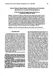
2.2 WORKING OF AN HVAC SYSTEM An HVAC system is designed to provide conditioned air to the occupied space, also called the ―conditioned‖ space, to maintain the desired level of comfort. To begin to explain how an HVAC system works let’s set some design conditions. First, we clean rooms. Examples of negative rooms are commercial kitchens, hospital intensive care units (ICU) and fume hood laboratories. Air Volume Using the roof top air handling unit as an example, the volume of air required to heat, ventilate, cool and provide good indoor air quality is calculated based on the 14
heating, cooling and ventilation loads. The air volumes are in units of cubic feet per minute (cfm). The total volume of air for this roof top unit (RTU) is calculated to be 5250 cfm. Constant volume supply air and return air fans (SAF and RAF) circulate the conditioned air to and from the occupied conditioned space. The total volume of return air back to the air handling unit is 4200 cfm. The difference between the amount of supply air (5250 cfm) and the return air (4200 cfm) is 1050 cfm. This is the ventilation air. It is used in the conditioned space for make-up air (MUA) for toilet exhaust and other exhaust systems. Ventilation air is also used for positive pressurization of the conditioned space, and for ―fresh‖ outside air to maintain good indoor air quality for the occupants. The return air, 4200 cfm, goes into the mixed air chamber (plenum). The return air is then mixed with 1050 cfm, which is brought in through the outside air (OA) dampers into the mixed air plenum. This 1050 cfm of outside air is the minimum outside air required for this system. It is 20% of the supply air (1050/5250). It mixes with the 4200 cfm of return air (80%, 4200/5250) to give mixed air (MA, 100%). Next, the 5250 cfm of mixed air then travels through the filters and into the coil sections. If more outside air than the minimum is brought into the system, perhaps for air-side economizer operation, any excess air is exhausted through exhaust air dampers (EA) to maintain the proper space pressurization. For example, if 2050 cfm is brought into the system through the OA dampers and 4200 cfm comes back through the return duct into the unit then 1000 cfm is exhausted through the exhaust air dampers (EA). This maintainsthe total supply cfm (5250) into the space and maintains the proper space pressurization. The airflow diagram looks like this:
Fig. 2.1 Air flow diagram
Where cfm
cubic feet per minute.
RA (return air) EA (exhaust air) MA (mixed air) OA (outside air) SA (supply air)
15
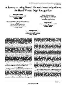
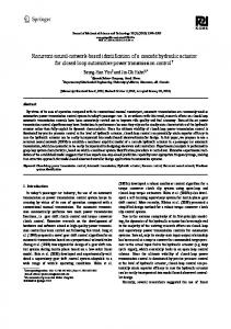
2.3 HVAC SYTEM MODEL The single-zone thermal system model shown in Fig. 2.2 is chosen for our analysis[21]. The system represents a simplification of an overall building climate control problem, but retains the distinguishing characteristics of an HVAC system. Fresh air enters the system at temperature T0(t) and volumetric flow rate f0(t) and is mixed with recirculated air at temperature T5(t) and flow rate f5(t). Air with temperature T1(t) and flow rate f(t). passes through the heat exchanger, where an amount of heat given by qhe(t) (positive for heating and negative for cooling) is exchanged with the air. The air and heat exchanger are assumed to have some capacitance, so that the resulting temperature T2(t) has a transient response. In addition, perfect mixing in the heat exchanger is assumed, so that the air temperature within and exiting the heat exchanger is T2(t). After being conditioned in the heat exchanger, the air passes into the thermal space. The capability of applying a space thermal load is included as ql(t). The temperature T3(t) of the space has a transient response due to the capacitance of the air and the thermal space. Perfect mixing in the thermal space is assumed, so that the air temperature within and exiting the space is T3(t). Air leaving the thermal space is drawn through the fan, after which a portion may be recirculated to mix with the fresh air and the remainder may be exhausted from the system. HVAC System model shown below Inlet Air
Flow Mixer 0
Heat Exchanger
1
2
T0 (t ), f 0 (t )
T2 (t )
Qhe (t )
q1 (t )
Energy Source
Return Air Damper
Thermal Space
Sr
Sq
5
ST
Controller
Sf
J
Exhaust Air
Flow splitter
4
Fan
Fig. 2.2 HVAC System model 16
f (t )
3
T3 (t )
The conditions within the system are regulated by a controller that provides signals to control the heat input in the heat exchanger, the volumetric airflow rate, and the position of the return air damper. The controller signals are depicted as thin lines and are denoted by S q, Sf and Sr. The signal ST denotes the temperature in the thermal space, while J denotes a cost associated with the performance of the system. Thermal losses between components are neglected and, thus, temperatures T4(t) and T5(t)
are equal to the temperature of the air
exiting the thermal space. In addition, infiltration and exfiltration effects are neglected and, thus, flow rates at locations 2–4 are equal to f(t).The humidity of the air is not considered, and transient effects in the flow splitter, mixer, fan, and heat exchanger are neglected. The system equations are derived from the conservation of energy principles and are given by
c pVhe c pVts
dT2 fc p (T1 T2 ) Qhe dt dT3 fc p (T2 T3 ) Ql dt
Where the parameters and variables are as described below. cp = constant pressure specific heat or air ( J/kg oC). f = volumetric airflow rate (m3/s). Qhe =heat input in the heat exchanger (W). Ql = thermal load on the room (W). t = time (s). Tref = desired thermal space temperature (oC). Ti = air temperature at location i (oC). Vhe = effective heat exchanger volume (m3). Vts = effective thermal space volume (m3). ρ = air density (kg/m3).
17
(2.1)
(2.2)
A lumped capacitance assumption is made, implying that the capacitance of the heat exchanger and the thermal space are accounted for in the effective heat exchanger and thermal space volumes. Statements of the conservation of mass and energy applied at the flow mixer yield T1 =T3 + ( T0 – T3)/r r=f ∕ f0
where
(2.3) (2.4)
is the system-to-fresh-air volumetric flow-rate ratio. For r=1, there is no recirculation and a once-through system is considered. The position of the return air damper as described by r is obtained from the values of f and f0 which are computed explicitly by the controller. Denoting x=[T2 T3]T and making the appropriate system equations x1
1 u1 (T0 X 2 )u3 ( X 2 X 1 )u2 Vhe c p
x2
1 Vts
Ql ( X 1 X 2 )u2 c p
(2.5)
(2.6)
Where u= [Qhe, f, f0]T.
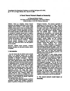
2.4 SIMULATION RESULTS The Heating, Ventilating, and Air-Conditioning (HVAC) Systems are a permanent part of everyday life in our industrialized society. The single-zone thermal system model shown in Fig. 2.2 is chosen for our analysis [21]. The system represents a simplification of an overall building climate control problem, but retains the distinguishing characteristics of an HVAC system. The HVAC system state equations shown above (2.5 and 2.6) are solved by RangeKutta method. For solving these system equations we considered the different variables and parameters have taken such as thermal load on the room (Ql), air density (ρ) and etc. Here the states x1 and x2 are in 0C with respect to time. These two states are identified by using different structures such as MLP, FLANN and ANFIS. All the simulations are carried out using MATLAB R2008a. The two desired states x1 and x2 shown in Fig.2.3.
18
Desired states x1 and x2 24 x1 x2
22
state values
20 18 16 14 12 10 0
10
20
30
40 time
50
60
70
80
Fig.2.3 HVAC System States in 0C
For the purposes of comfort and hygiene, the minimum allowable value of u3, the outside air volumetric flow rate, is set at 0.0354 m3/ s[22]. The equilibrium states of the system are u3T0 x1EQ x2 EQ
u1 c p
u3
(2.7)
Since this is an underdetermined case, an infinite number of combinations of u1 and u2 provide the same steady-state output and the system does not possess a unique inverse. The ranges of the control variables are defined as Qhe=Є[-4000,4000]W
(2.8)
f, f0Є[0.0354,2]m3/s.
(2.9)
and
The value of u3 can never exceed the value of u2 , due to conservation of mass principles. Thus, the controller must command values for these inputs that satisfy the following condition: u2 ≥ u3.
(2.10)
The operating ranges of the system states and outside air temperature are assumed to be x1 Є[5,35] 0C or [41,95] 0F x2,T0 Є[10,30] 0C or [50,86] 0F
19
(2.11) (2.12)
and the range of the reference temperature is assumed be Tref Є [17,23] 0C or [62.6, 73.4] 0F
(2.13)
In order to most effectively use u3, the controller must have information as to whether the outside air temperature is higher or lower than the desired room temperature. Thus, an additional input variable called Tdiff is introduced, Where Tdiff = Tref –T0
(2.14)
It is assumed that T0 can be measured accurately with an inexpensive temperature sensor. In order to determine the ranges of the changes in the states over a sample period of Ts=10 s, the state equations (3.5) and (3.6) are integrated from 0–10 s, using 1000 random initial conditions satisfying (3.8)–(3.12). Histograms for Δx1 and Δx2. Based on the extreme values of Δx1 and Δx2. The ranges for the changes in the states are assumed to be Δx1 Є [-13.0, 13.0] 0C
(2.15)
Δx2 Є [-1.5, 1.5] 0C
(2.16)
The range of control signals using assumptions (2.11)–(2.13), (2.15), and (2.16) will be used to train the neural network to learn the HVAC thermal dynamics.
2.5 HEATING AND COOLING Heat is energy in the form of molecules in motion. Heat flows from a warmer substance to a cooler substance. Heat energy flows downhill! Heat does not raise, heated air rises! Temperature is the level of heat (energy). The lowest temperature is minus 460°F. The sun’s temperature is approximately 27,000,000°F. The temperatures associated with most HVAC systems range from 0°F to 250°F. Most people feel comfortable if the indoor air temperature is between 68°F and 78°F.
2.5.1 Standard Temperatures on the Fahrenheit and Celsius Scales Freezing point of (pure) water is: 32 degrees Fahrenheit (32°F) and zero degrees Celsius (0°C). Boiling point of (pure) water is: 212 degrees Fahrenheit (212°F) and 100 degrees Celsius (100°C).
20
Temperature Conversions for Fahrenheit and Celsius °C = (°F - 32) ÷ 1.8 °F = 1.8 (°C) + 32 The following is a quick reference for estimating and converting everyday temperatures from Celsius to Fahrenheit: 0°C is 32°F 16°C is approximately 61°F 28°C is approximately 82°F 37°C is 98.6°F 100°C is 212°F Absolute Temperatures The Fahrenheit absolute scale is the Rankine (°R) scale. The Celsius absolute scale is the Kelvin (°K) scale. Absolute zero is minus 460°F and 0°R, or minus 273°C and 0°K. The Fahrenheit/Celsius and the Rankine/Kelvin scales are used interchangeably to describe equipment and fundamentals of the heating and air conditioning industry.
2.5.2 Heat and Temperature Heat is energy in the form of molecules in motion. As a substance becomes warmer, its molecular motion and energy level (temperature) increases. Temperature describes the level of heat (energy) with reference to no heat. Heat is a positive value relative to no heat. Because all heat is a positive value in relation to no heat, cold is not a true value. It is really an expression of comparison. Cold has no number value and is used by most people as a basis of comparison only. Therefore, warm and hot are comparative terms used to describe higher temperature levels. Cool and cold are comparative terms used to describe lower temperature levels. The Fahrenheit scale is the standard system of temperature measurement used in the United States. However, the U.S. is one of the few countries in the world still using this system. Most countries use the metric temperature measurement system, which is the Celsius scale. The Fahrenheit and Celsius scales are currently used interchangeably in the U.S. to describe equipment and fundamentals in the heating, ventilating and air conditioning industry.
21
2.5.3 Heat Transfer Heat naturally flows from a higher energy level to a lower energy level. In other words, heat travels from a warmer substance to a cooler substance. When there is a temperature difference between two substances, heat transfer will occur. In fact, temperature difference is the driving force behind heat transfer. The greater the temperature difference, the greater the heat transfer.
2.5.4 Types of Heat Transfer The three types of heat transfer are conduction, convection and radiation. Conduction Conduction heat transfer is heat energy traveling from one molecule to another. A heat exchanger in an HVAC system or home furnace uses conduction to transfer heat. Your hand touching a cold wall is an example of heat transfer by conduction from your hand to the wall. However, heat does not conduct at the same rate in all materials. For example, all HVAC copper conducts at a different rate than iron or aluminum, etc. Convection Heat transfer by convection is when some substance that is readily movable such as air, water, steam, or refrigerant moves heat from one location to another. Compare the words ―convection‖ (the action of conveying) and ―convey‖ (to take or carry from one place to another). An HVAC system uses convection in the form of air, water, steam and refrigerants in ducts and piping to convey heat energy to various parts of the system. When air is heated, it rises; this is heat transfer by ―natural‖ convection. ―Forced‖ convection is when a fan or pump is used to convey heat in fluids such as air and water. For example, many large buildings have a central heating plant where water is heated and pumped throughout the building to the final heated space. Fans then move heated air into the conditioned space. Radiation Heat transferred by radiation travels through space without heating the space. Radiation or radiant heat does not transfer the actual temperature value. The first solid object that the heat rays encounter absorbs the radiant heat. A portable electric space heater that glows red-hot is an example of heat transfer by radiation. As the electric heater coil glows red-hot it radiates heat into the room. The space heater does not heat the air (the space)—instead it heats the solid objects that come into contact with the heat rays. Any heater that glows has the same effect. However, radiant heat diminishes by the square of the distance traveled; therefore, 22
space heaters must be placed accordingly. Another good example of radiant heat is the sun; the sun heats the earth, but not the air around the earth. The sun is also a good example of diminishing heat. The earth does not experience the total heat of the sun because the sun is some 93 million miles from the earth.
2.5.5 Ventilating The ventilation requirement is 1050 cfm. 1050 cfm of outside air is brought in through the outside air (OA) dampers into the mixed air plenum. This 1050 cfm of outside air mixes with the 4200 cfm of return air to form 5250 cfm of mixed air, which goes through the coil(s) and becomes supply air.
2.5.6 Cooling For this system, the total heat given off by the people, lights and equipment in the conditioned space plus the heat entering the space through the outside walls, windows, doors, roof, etc., and the heat contained in the outside ventilation air will be approximately 154,000 Btu/hr. A ton of refrigeration (TR) is equivalent to 12,000 Btu/hr of heat. Therefore, this HVAC system requires a chiller that can provide approximately 13 tons of cooling (154,000 Btu/hr ÷ 12000 Btu/hr/ton = 12.83 TR) To maintain the proper temperature and humidity in the conditioned space the cooling cycle is this: The supply air (which is 20°F cooler than the air in the conditioned space) leaves the cool ing coil and goes through the heating coil (which is off), through the supply air fan, down the duct and into the conditioned space. The cool supply air picks up heat in the conditioned space. The warmed air makes its way into the return air inlets, then into the return air duct and back to the air handling unit. The return air goes through the return air fan into the mixed air chamber and mixes with the outside air. The mixed air goes through the filters and into the cooling coil. The mixed air flows through the cooling coil where it gives up its heat into the chilled water tubes in the coil. This coil also has fins attached to the tubes to facilitate heat transfer. The cooled supply air leaves the cooling coil and the air cycle repeats. The water, after picking up heat from the mixed air, leaves the cooling coil and goes through the chilled water return (CHWR) pipe to the water chiller’s evaporator. The ―warmed‖ water flows into the chiller’s evaporator—sometimes called the water cooler—where it gives up the heat from the mixed air into the refrigeration system. The newly ―chilled‖ water leaves the evaporator, goes through the chilled water pump (CHWP) and is pumped through the chilled water supply (CHWS) piping into the cooling coil to pick up heat from the mixed air and the water cycle repeats. The evaporator is 23
a heat exchanger that allows heat from the chilled water return (CHWR) to flow by conduction into the refrigerant tubes. The liquid refrigerant in the tubes ―boils off‖ to a vapor removing heat from the water and conveying the heat to the compressor and then to the condenser. The heat from the condenser is conveyed to the cooling tower through the condenser water in the condenser return (CWR) pipe. As the condenser water cascades down the tower, outside air is drawn across the cooling tower removing heat from the water through the process of evaporation. The ―cooled‖ condenser water falls to the bottom of the tower basin and is pumped from the tower through the condenser water pump (CWP) and back to the condenser in the condenser water supply piping (CWS) and the cycle repeats.
2.6 HEATING SYSTEMS For over 10,000 years, man has used fire to warm himself. In the beginning, interior heating was just an open fire, but comfort and health was greatly improved by finding a cave with a hole at the top. Later, fires were contained in hearths or sunken beneath the floor. Eventually, chimneys were added which made for better heating, comfort, health, and safety and also allowed individuals to have private rooms. Next, came stoves usually made of brick, earthenware, or tile. In the 1700s, Benjamin Franklin improved the stove, the first steam heating system was developed, and a furnace for warm-air heating used a system of pipes and flues and heated the spaces by gravity flow. In the 1800s, high speed centrifugal fans and axial flow fans with small, alternating current electric motors became available and highpressure steam heating systems were first used. The 1900s brought the Scotch marine boiler and positive-pressure hydronic circulating pumps that forced hot water through the heating system. The heating terminals were hot water radiators, which were long, low, and narrow, as compared to steam radiators, and allowed for inconspicuous heating. Centrifugal fans were added to furnaces in the 1900s to make forced-air heating systems.
2.7 VENTILATING SYSTEMS In occupied buildings, carbon dioxide, human odors and other contaminants such as volatile organic compounds (VOC) or odors and particles from machinery and the process function need to be continuously removed or unhealthy conditions will result. Ventilation is the process of supplying ―fresh‖ outside air to occupied buildings in the proper amount to offset the contaminants produced by people and equipment. In many instances, local building codes, association guidelines, or government or company protocols stipulate the amount of 24
ventilation required for buildings and work environments. Ventilation systems have been around for a long time. In 1490, Leonardo da Vinci designed a water driven fan to ventilate a suite of rooms. In 1660, a gravity exhaust ventilating system was used in the British House of Parliament. Then, almost two hundred years later, in 1836, the supply air and exhaust air ventilation system in the British House of Parliament used fans driven by steam engines. Today, ventilation guidelines are approximately 15 to 25 cfm (cubic feet per minute) of air volume per person of outside air (OA) for non-smoking areas, 50 cfm for smoking areas. Ventilation air may also be required as additional or ―make-up‖ air (MUA) for kitchen exhausts, fume hood exhaust systems, and restroom and other exhaust systems. Maintaining room or conditioned space pressurization (typically +0.03 to +0.05 inches of water gage) in commercial and institutional buildings is part of proper ventilation. Figure 4-10 shows 20% of the total supply air is ventilation outside air (OA) and 80% is return air (RA). The outside air is brought (or forced) into the mixed air plenum by the action of the supply air fan. The outside air coming through the outside damper is mixed with the return air from the conditioned space. The return air dampers control the amount of return air. If the room pressure is too high, the exhaust air (EA) dampers open to let some of the return air escape to the outside, which relieves some of the pressure in the conditioned space. Exhaust air dampers are also called relief air dampers.
2.8 AIR CONDITIONING SYSTEMS Brooklyn, New York, was the place, and 1902 was the year the first truly successful air conditioning system for room temperature and humidity control was placed into operation. But first it took the engineering innovations of Willis Carrier to advance the basic principles of cooling and humidity control and design the system. Cooling air had already been done successfully but it was only part of the air conditioning problem. The other part was how to regulate space humidity. Carrier recognized that drying the air could be accomplished by saturating it with chilled water to induce condensation. In 1902, Carrier built the first air conditioner to combat both temperature and humidity. The air conditioning unit was installed in a printing company and chilled coils were used in the machine to cool the air and lower the relative humidity to 55%. Four years later, in 1906, Carrier was granted a patent for his air conditioner the ―Apparatus for Treating Air.‖ However, Willis Carrier did not invent the very first system to cool an interior structure nor interestingly, did he come up with the term ―air conditioning.‖ It was Stuart Cramer, a textile engineer, who coined the term ―air 25
conditioning.‖ Mr.Cramer used ―air conditioning‖ in a 1906 patent for a device that added water vapor to the air. In 1911, Mr. Carrier, who is called the ―father of air conditioning,‖ presented his ―Rational Psychrometric Formulae‖ to the American Society of Mechanical Engineers. Today, the formula is the basis in all fundamental psychometric calculations for the air conditioning industry. Though Willis Carrier did not invent the first air conditioning system, his cooling and humidity control system and psychrometric calculations started the science of modern psychrometrics and air conditioning. As already mentioned, air ―cooling‖ was only part of the answer. The big problem was how to regulate indoor humidity. Carrier’s air conditioning invention addressed both issues and has made many of today’s products and technologies possible. In the 1900s, many industries began to flourish with the new ability to control the indoor environmental temperature and humidity levels in both occupied and manufacturing areas. Today, air conditioning is required in most industries and especially in ones that need highly controllable environments, such as clean environment rooms (CER) for medical or scientific research, product testing, and sophisticated computer and electronic Component manufacturing.
26
CHAPTER 3 SYSTEM IDENTIFICATION USING ARTIFICIAL NEURAL NETWORKS
3.1 INTRODUCTION Nonlinear system identification of a complex dynamic plant has potential applications in many areas such as control, communication, power system, instrumentation, pattern recognition and classification. Because of the function approximation properties and learning capability, Artificial Neural Networks (ANN’s) have become a powerful tool for these complex applications. The ANN’s are capable of generating complex mapping between the input and the output space and thus, arbitrarily complex nonlinear decision boundaries can be formed by these networks. An artificial neural network basically consists a number of computing elements, called neurons that perform the weighted sum of the input signal and the connecting weight. The sum is added with the bias or threshold and the resultant signal is then passed through a non-linear element such as tanh(. ) type. Each neuron is associated with three parameters on whose learning of neuron can be adjusted; these are the connecting weights, the bias and the slope of the non-linear function. From the structural point of view, a neural network (NN) may be single layer or it may be multi-layer. In multi-layer structure, there may be more than one hidden layers and there is one or many artificial neurons in each layer and for a practical case there may be a number of layers. Each neuron of one layer is connected to each and every neuron of the next layer. A neural network is a massively parallel distributed processor made up of simple processing unit, which has a natural property for storing experimental knowledge and making it available for use. It resembles the brain in two types 1. Knowledge is acquired by the network from its environment through a learning process. 2. Interneuron connection strengths, known as synaptic weights, are used to store the acquired knowledge. Artificial Neural Networks (ANN) has emerged as a powerful learning technique to perform complex tasks in highly nonlinear dynamic environments. Some of the prime advantages of using ANN models are their ability to learn based on optimization of an appropriate error function and their excellent performance for approximation of nonlinear function [3]. At present, most of the work on system identification using neural networks are based on multilayer feed-forward neural networks with back propagation learning or more efficient variations of this algorithm [18] ,[1].On the otherhand the Functional link ANN(FLANN) originally proposed by Pao [12] is a single layer structure with functionally 28
mapped inputs. Wang and Chen [19] have presented a fully automated recurrent neural network (FARNN) that is capable of self-structuring its network in a minimal representation with satisfactory performance for unknown dynamic system identification and control.
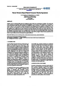
3.2 NEURON STRUCTURE In 1958, Rosenblatt demonstrated some practical applications using the perceptron [20]. The perceptron is a single level connection of McCulloch-Pitts neurons sometimes called singlelayer feed-forward networks. The network is capable of linearly separating the input vectors into pattern of classes by a hyper plane. A linear associative memory is an example of a single-layer neural network. In such an application, the network associates an output pattern (vector) with an input pattern (vector), and information is stored in the network by virtue of modifications made to the synaptic weights of the network. b(n) x1 x2 . . .
f(.)
y(n)
. xN
Fig 3.1 Neuron Structure
The structure of a single neuron is presented in Fig. 3.1. An artificial neuron involves the computation of the weighted sum of inputs and threshold [3]. The resultant signal is then passed through a non-linear activation function. The output of the neuron may be represented as,
𝑦 𝑛 =𝑓
𝑁 𝑗 =1 𝑤𝑗
𝑛 𝑥𝑗 𝑛 + 𝑏 𝑛
(3.1)
where, b(n) = threshold to the neuron is called as bias, wj(n) = weight associated with the jth input, and N = no. of inputs to the neuron.
3.2.1 Activation Functions and Bias The perceptron internal sum of the inputs is passed through an activation function, which can be any monotonic function. Linear functions can be used but these will not contribute to a non-linear transformation within a layered structure, which defeats the purpose of using a neural filter implementation. A function that limits the amplitude range and limits the output strength of each perceptron of a layered network to a defined range in a non-linear manner 29
will contribute to a nonlinear transformation. There are many forms of activation functions, which are selected according to the specific problem. All the neural network architectures employ the activation function [3, 27] which defines as the output of a neuron in terms of the activity level at its input (ranges from -1 to 1 or 0 to 1). Table 3.1 summarizes the basic types of activation functions. The most practical activation functions are the sigmoid and the hyperbolic tangent functions. This is because they are differentiable.
NAME
MATHEMATICAL REPRESENTATION
Linear
𝑓(𝑥) = 𝑘𝑥
Step
𝑓 𝑥 =
𝛼, 𝑖𝑓 𝑥 ≥ 𝑘 𝛽, 𝑖𝑓 𝑥 < 𝑘
Sigmoid
𝑓 𝑥 =
1 ,𝛼 > 0 1 + 𝑒 −𝛼𝑥
Hyperbolic Tangent
𝑓 𝑥 =
1 − 𝑒 −𝛾𝑥 ,𝛾 > 0 1 + 𝑒 −𝛾𝑥
Gaussian
𝑓 𝑥 =
1 2𝜋𝜎 2
𝑒
−
𝑥−𝜇 2 2𝜎 2
Table 3.1 Types of Activation Functions
The bias gives the network an extra variable and the networks with bias are more powerful than those of without bias. The neuron without a bias always gives a net input of zero to the activation function when the network inputs are zero. This may not be desirable and can be avoided by the use of a bias.
30
3.2.2 Learning Technique: The property that is of primary significance for a neural network is that the ability of the network to learn from its environment, and to improve its performance through learning. The improvement in performance takes place over time in accordance with some prescribed measure. A neural network learns about its environment through an interactive process of adjustments applied to its synaptic weights and bias levels. Ideally, the network becomes more knowledgeable about its environment after each iteration of learning process. Hence we define learning as: ―It is a process by which the free parameters of a neural network are adapted through a process of stimulation by the environment in which the network is embedded.‖ The processes used are classified into two categories as described in [3]: (i) Supervised Learning (Learning With a Teacher) (ii) Unsupervised Learning (Learning without a Teacher) (i)
Supervised Learning:
We may think of the teacher as having knowledge of the environment, with that knowledge being represented by a set of input-output examples. The environment is, however unknown to neural network of interest. Suppose now the teacher and the neural network are both exposed to a training vector, by virtue of built-in knowledge, the teacher is able to provide the neural network with a desired response for that training vector. Hence the desired response represents the optimum action to be performed by the neural network. The network parameters such as the weights and the thresholds are chosen arbitrarily and are updated during the training procedure to minimize the difference between the desired and the estimated signal. This updation is carried out iteratively in a step-by-step procedure with the aim of eventually making the neural network emulate the teacher. In this way knowledge of the environment available to the teacher is transferred to the neural network. When this condition is reached, we may then dispense with the teacher and let the neural network deal with the environment completely by itself. This is the form of supervised learning. By applying this type of learning technique, the weights of neural network are updated by using LMS algorithm. The update equations for weights are derived as LMS [3]: 𝑤𝑗 𝑛 + 1 = 𝑤𝑗 𝑛 + 𝜇∆𝑤𝑗 (𝑛) (ii)
(3.2)
Unsupervised Learning:
In unsupervised learning or self-supervised learning there is no teacher to over-see the learning process, rather provision is made for a task independent measure of the quantity of
31
representation that the network is required to learn, and the free parameters of the network are optimized with respect to that measure. Once the network has become turned to the statistical regularities of the input data, it develops the ability to form the internal representations for encoding features of the input and thereby to create new classes automatically. In this learning the weights and biases are updated in response to network input only. There are no desired outputs available. Most of these algorithms perform some kind of clustering operation. They learn to categorize the input patterns into some classes.
3.3 MULTILAYER PERCEPTRON In the multilayer neural network or multilayer perceptron (MLP), the input signal propagates through the network in a forward direction, on a layer-by-layer basis. This network has been applied successfully to solve some difficult and diverse problems by training in a supervised manner with a highly popular algorithm known as the error back-propagation algorithm [3]. The scheme of MLP using four layers is shown in Fig.3.2. 𝑥𝑖 (𝑛) represents the input to the network, 𝑓𝑗 and 𝑓𝑘 represent the output of the two hidden layers and 𝑦𝑖 (𝑛) represents the output of the final layer of the neural network. The connecting weights between the input to the first hidden layer, first to second hidden layer and the second hidden layer to the output layers are represented by respectively +1
wjk
+1
wij +1
wkl
Input signal xi(n)
Output signal yi(n)
… … … Input Layer (Layer-1)
… … …
… … …
Second Hidden Layer (Layer-3)
First Hidden Layer-2 Fig 3.2(Layer-2) Structure of Multilayer Perceptron 32
Output Layer (Layer-4)
If P1 is the number of neurons in the first hidden layer, each element of the output vector of first hidden layer may be calculated as, 𝑓𝑗 = 𝜑𝑗
𝑁 𝑖=1 𝑤𝑖𝑗 𝑥𝑖
𝑛 + 𝑏𝑗 , 𝑖 = 1,2, … 𝑁, 𝑗 = 1,2, … 𝑃1
(3.3)
where bj is the threshold to the neurons of the first hidden layer, N is the no. of inputs and 𝜑 is the nonlinear activation function in the first hidden layer chosen from the Table 3.1. The time index n has been dropped to make the equations simpler. Let P2 be the number of neurons in the second hidden layer. The output of this layer is represented as, fk and may be written as 𝜑𝑘
𝑃1 𝑗 =1 𝑤𝑗𝑘 𝑓𝑗
+ 𝑏𝑘 , 𝑘 = 1,2, … . 𝑃2
(3.4)
where, bk is the threshold to the neurons of the second hidden layer. The output of the final output layer can be calculated as 𝑦𝑙 𝑛 = 𝜑𝑙
𝑃2 𝑘=1 𝑤𝑘𝑙 𝑓𝑘
+ 𝑏𝑙 , 𝑙 = 1,2, … 𝑃3
(3.5)
where, bl is the threshold to the neuron of the final layer and P3 is the no. of neurons in the output layer. The output of the MLP may be expressed as 𝑦𝑙 𝑛 = 𝜑𝑙
𝑃2 𝑘=1 𝑤𝑘𝑙
𝜑𝑘
𝑃1 𝑗 =1 𝑤𝑗𝑘
𝜑𝑗
𝑁 𝑖=1 𝑤𝑖𝑗 𝑥𝑖
𝑛 + 𝑏𝑗
+ 𝑏𝑘
+ 𝑏𝑙
(3.6)
3.3.1 Back Propagation Algorithm x1
x2
yl(n) -
Back-Propagation Algorithm
+ dl(n) el(n)
Fig 3.3 Neural Network with Back Propagation Algorithm
An MLP network with 2-3-2-1 neurons (2, 3, 2 and 1 denote the number of neurons in the input layer, the first hidden layer, the second hidden layer and the output layer respectively) 33
with the back-propagation (BP) learning algorithm, is depicted in Fig.3.3. The parameters of the neural network can be updated in both sequential and batch mode of operation. In BP algorithm, initially the weights and the thresholds are initialized as very small random values. The intermediate and the final outputs of the MLP are calculated by using (3.3), (3.4), and (3.5.) respectively. The final output 𝑦𝑙 (𝑛) at the output of neuron l, is compared with the desired output 𝑑 𝑛 and the resulting error signal 𝑒 𝑛 is obtained as 𝑒𝑙 𝑛 = 𝑑 𝑛 − 𝑦𝑙 𝑛
(3.7)
The instantaneous value of the total error energy is obtained by summing all error signals over all neurons in the output layer, that is 𝜉 𝑛 =
1
𝑃3 2 𝑙=1 𝑒𝑙 (𝑛)
2
(3.8)
where P3 is the no. of neurons in the output layer. This error signal is used to update the weights and thresholds of the hidden layers as well as the output layer. The reflected error components at each of the hidden layers is computed using the errors of the last layer and the connecting weights between the hidden and the last layer and error obtained at this stage is used to update the weights between the input and the hidden layer. The thresholds are also updated in a similar manner as that of the corresponding connecting weights. The weights and the thresholds are updated in an iterative method until the error signal become minimum. For measuring the degree of matching, Squared error cannot be considered as the network may have multiple outputs and Root Mean Square Error (RMSE) cause over fitting of the model and the weights may not converge. So the Mean Square Error (MSE) is taken as a performance measurement. The weights are using the following formulas, 𝑤𝑘𝑙 𝑛 + 1 = 𝑤𝑘𝑙 𝑛 + ∆𝑤𝑘𝑙 𝑛
(3.9)
𝑤𝑗𝑘 𝑛 + 1 = 𝑤𝑗𝑘 𝑛 + ∆𝑤𝑗𝑘 𝑛
(3.10)
𝑤𝑖𝑗 𝑛 + 1 = 𝑤𝑖𝑗 𝑛 + ∆𝑤𝑖𝑗 𝑛
(3.11)
∆𝑤𝑘𝑙 𝑛 = −2𝜇
𝜕𝜉 (𝑛) 𝜕𝑤 𝑘𝑙 𝑛
= 𝜇𝑒(𝑛)𝜑𝑙′
= 𝜇𝑒(𝑛)
𝑃2 𝑘=1 𝑤𝑘𝑙 𝑓𝑘
𝑑𝑦 𝑙 (𝑛) 𝑑𝑤 𝑘𝑙 𝑛
+ 𝑏𝑙
𝑓𝑘
where, µ is the convergence coefficient (0