A Symbolic Model Checking Framework for Hierarchical Systems Truong Khanh Nguyen∗ , Jun Sun† , Yang Liu∗ and Jin Song Dong∗ ∗ School of Computing, National University of Singapore Email: {truongkhanh,liuyang,dongjs}@comp.nus.edu.sg † Singapore University of Technology and Design Email:
[email protected]
Abstract—BDD-based symbolic model checking is capable of verifying systems with a large number of states. In this work, we report an extensible framework to facilitate symbolic encoding and checking of hierarchical systems. Firstly, a novel library of symbolic encoding functions for compositional operators (e.g., parallel composition, sequential composition, choice operator, etc.) are developed so that users can apply symbolic model checking techniques to hierarchical systems with little knowledge of symbolic encoding techniques (like BDD or CUDD). Secondly, as the library is language-independent, we build an extensible framework with various symbolic model checking algorithms so that the library can be easily applied to encode and verify different modeling languages. Lastly, the applicability and scalability of our framework are demonstrated by applying the framework in the development of symbolic model checkers for three modeling languages as well as a comparison with the NuSMV model checker.
I. S YSTEM OVERVIEW Binary Decision Diagram (BDD) based symbolic model checking is capable of verifying systems with a large number of states. Its effectiveness has been evidenced by the recent success of the Intel i7 project, where BDD techniques have been applied to verify the i7 processor [3]. Currently, symbolic model checking techniques are mostly applied to simple transitions system with little structure. Complex systems on the other hand are often hierarchical, where high level system components are composed by subcomponents in many different ways (e.g. choice, parallel composition, sequential composition, etc). Many languages are dedicated to model hierarchical systems such as Statecharts (where hierarchy is introduced through compositional states), process algebras like CSP (where hierarchy is introduced through processes), or programming languages like C++ or Java (where hierarchy is introduced through classes). These languages are also distinguished from each other in many aspects, e.g., how different components communicate. Applying BDD-based model checking to models specified using these languages is highly non-trivial. The input language of the popular NuSMV model check has limited support for modular hierarchical descriptions. For instance, it supports only parallel composition and interleaving but not other useful composition operators like choice, interrupt, etc. Modeling hierarchical systems in NuSMV could thus be difficult. In this work, we report a model
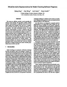
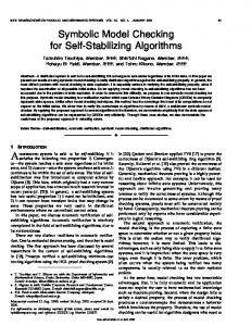
checking framework designed to facilitate application of BDD technique to fully hierarchical systems. Our framework aims to provide a unified solution so that systems modeled using compositional languages can be encoded and verified symbolically with minimum efforts. The first component of our framework is a novel library (based on the CUDD package) of symbolic encoding functions for system compositions. The library covers common compositional system behaviors patterns and comes with well-designed interfaces so that minimum knowledge on BDD is required in order to apply the encoding functions. System encoding in our framework works by firstly identifying and encoding primitive system components and then repeatedly composing encoded system components using the composition functions. We assume that primitive system components (e.g., a compositional state which contains no other compositional states, or a process which invokes no other processes) are in the form of finite state machines, which can be encoded using BDD in the standard way. In order to build a generally useful framework, we take into account different ways of communication between system components: communication through shared memory; synchronous/asynchronous channel communication; and multi-party barrier synchronization (e.g., CSP-style). Next, with process algebras like CSP and CCS in mind, a rich set of system composition functions are provided. Using these functions, encoded system components can be composed in a variety of ways, including parallel composition, sequential composition, interrupt, choice, etc. A symbolic encoding of a hierarchical system thus can be gradually obtained from bottom up using the provided functions in the library. In order to further ease the application of our library, we build a framework so that the library can be easily applied to encode and verify different modeling languages. The framework adopts a layered architecture design as shown in Fig. 1. The first layer denotes the application domains and the second layer denotes the corresponding modeling languages of the application domains. Each language is encapsulated as a plug-in module by following the design guildine1 . After compilation, input models are parsed into internal representations (IR), which implement the opera1 This
can be found in PAT user manual Section 5.1.
Modeling
LTS Module
Abstraction
Concurrent Systems, Sensor Networks, Hierarchical Probabilistic Systems...
Domain-specific Abstraction: data abstraction, zone abstraction, environment abstraction, etc.
NesC Module
Symbolic Encoding
Probabilistic Module
...
Operational Semantic
Symbolic Representation:
Simulator
Analysis
Binary Decision Diagram
Counterexample Generator
Symbolic Verification Algorithms Deadlock, Reachability, LTL Symbolic Model Checking
Figure 1.
Architecture Design
tional semantics. This IR can be used by the simulator for simulating the system behaviors. To perform symbolic model checking, our BDD library is used to generate the encoding of the IR in a compositional way. Furthermore, a set of symbolic model checking algorithms are developed to verify properties like deadlock-freeness, reachability and linear temporal logics. If the verification result is false, the boolean variable assignment satisfying the Boolean model is returned to the counterexample generator, which will translate the assignment to a counterexample in the form of system execution trace for users to locate the bug. We have developed three symbolic model checkers in our framework based on our library, i.e., LTS module for modeling hierarchical systems by composing label transition systems, CSP module for modeling concurrent system modeled using communicating sequential process, and NesC module for modeling sensor networks based on NesC language. This framework has been realized as a major part of the PAT tool [7], which is a self-contained model checker to support composing, simulating and reasoning of different application domains. PAT comes with user friendly interfaces, featured model editor and animated simulator. Most importantly, it supports two different model checking techniques, i.e., explicit model checking and symbolic model checking. The work presented in this paper provides support of symbolic model checking in the PAT framework. II. E NCODING H IERARCHICAL S YSTEMS This section explains how primitive system components are encoded and then how encoded components can be composed in a hierarchical manner. A. Encoding Primitive System Components Without loss of generality, we assume that a primitive system component takes the form of a finite state machine. A finite state machine has finitely many local control states and local variables (with finite domains). A transition is a link from one local control state to another state, which is labeled with a guard condition (constituted by global/local variables), an optional event and a transaction. An event
can be a channel input or output, or a (compound) name constituted by local variables as well as global variables. We note that an event (besides channel input/output) can serve as a synchronization barrier (see later on parallel composition II-B). A transaction is a sequential program which possibly updates global/local variables. Note that a finite state machine may communicate with others in different ways, e.g. shared variables, event synchronization or channel communication. Finite state machines are encoded using BDD in the standard way. That is, a BDD is used to encode symbolically the system configuration including valuation of variables, channels, etc. A transition is encoded using two sets of − − Boolean variables → x and → x 0 , which represent system configurations before and after the transaction. Transactions are − − encoded as BDDs constituted by → x and → x 0 . For instance, if the transaction is a simple assignment of the form y := expr, − then the encoding would denote that variables in → x 0 which encodes y is equivalent to value of expr (based on variables − − in → x ) and the rest of → x 0 remains unchanged. Other program constructs like if -then-else or while-do 2 are encoded similarly (refer to [5] for details). An encoded transition is − in the form: g ∧ e ∧ t such that g (over → x ) is an encoded − guard condition; e is an encoded event and t (over → x and 0 → − x ) is an encoded transaction. A BDD encoding of a finite state machine, which is referred to as a BDD machine, is a tuple B = → − − → − (V ,→ v , Init, Trans, Out, In) where V is a set of unprimed Boolean variables encoding global variables, event names −v is the variables for local variables and channel names3 ; → → − −v and local control states; Init is a formula over V and → encoding the initial valuation of the variables; Trans is a set of encoded transitions; Out (In) is a set of encoded transitions labeled with synchronous channel output (input). Note that transitions in Out and In are to be matched by corresponding input/output from the environment or equivalently other system components. B. Composing BDD Machines In this section, we show how to compose BDD machines in order to model hierarchical systems. We fix two BDD ma→ − − chines Bi = ( V , → v i , Initi , Transi , Outi , Ini ) where i ∈ {0, 1} −v 0 and → −v 1 are disjoint in the following. We assume that → → − (otherwise variable renaming is necessary). Note that V is always shared. The following shows some of the most common composition patterns as examples. Refer to [5] for the complete list. Parallel Composition: The parallel composition of two components B0 and B1 is a BDD machine → − − (V ,→ v , Init, Trans, Out, In) such that v = v0 ∪ v1 ; Init = Init0 ∧ Init1 ; and the encoded transitions are defined as 2 Encoding 3 Note
these programming features are not trivial. − → that V is fixed before encoding the system components.
−v 1−i = follows. Out contains a transition gi ∧ ei ∧ ti ∧ (→ → −v 0 ) if gi ∧ ei ∧ ti is a transition in Outi . For instance, 1−i the composition may perform a synchronous channel output action if B1 can perform such action and the local state of B0 remains unchanged. In contains a transition gi ∧ ei ∧ −v 1−i = → −v 0 ) if gi ∧ ei ∧ ti is a transition in Ini . ti ∧ (→ 1−i Trans contains three kinds of transitions. •
•
•
Local transitions: if gi ∧ ei ∧ ti is a transition in Transi and ei is an asynchronous channel input/output or ei is an event which is not to be synchronized, Trans −v 1−i = → −v 0 ). contains a transition gi ∧ ei ∧ ti ∧ (→ 1−i Synchronous channel communication: if gi ∧ ei ∧ ti is a transition in Outi and g1−i ∧ e1−i ∧ t1−i is a transition in In1−i , Trans contains a transition gi ∧ g1−i ∧ ei ∧ e1−i ∧ ti ∧ t1−i 4 . Barrier synchronization: if gi ∧ ei ∧ ti is a transition in Transi and g1−i ∧ ei ∧ t1−i is a transition in Trans1−i and ei is a synchronization barrier, Trans contains a transition gi ∧ g1−i ∧ ei ∧ ti ∧ t1−i .
Choice: An unconditional choice between B0 and B1 is → − − a BDD machine ( V g , → v , Init, Trans, Out, In) such that v = v0 ∪ v1 ∪ {choice} where choice is a fresh Boolean variable, choice = i means Bi is selected; Init = Init0 ∧ Init1 , the variable choice is not initialized and thus B0 and B1 can be randomly selected; and the encoded transitions are defined as follows. Out contains a transition (choice = i) ∧ gi ∧ −v 1−i = → −v 0 ) if gi ∧ ei ∧ ti is ei ∧ ti ∧ (choice0 = i) ∧ (→ 1−i a transition in Outi . In contains a transition (choice = i) ∧ −v 1−i = → −v 0 ) if gi ∧ ei ∧ ti gi ∧ ei ∧ ti ∧ (choice0 = i) ∧ (→ 1−i is a transition in Ini . Trans contains a transition (choice = −v 1−i = → −v 0 ) if i) ∧ gi ∧ ei ∧ ti ∧ (choice0 = i) ∧ (→ 1−i gi ∧ ei ∧ ti is a transition in Transi . In literature, there are other choices like external/internal choice or conditional choice, all of which are supported similarly. Sequential Composition: A system where B1 executes whenever B0 terminates is a BDD program → − − ( V g, → v , Init, Trans, Out, In) such that v = v0 ∪ v1 ∪ {terminated} where terminated is a fresh Boolean variable; Init = Init0 ∧ Init1 ∧ (terminated = false). Out contains a transition (terminated = false) ∧ g0 ∧ e0 ∧ t0 ∧ −v 1 = → −v 0 ) if g0 ∧ e0 ∧ t0 is a (terminated0 = false) ∧ (→ 1 transition in Out0 . Out contains a transition (terminated = −v 0 = → −v 0 ) true) ∧ g1 ∧ e1 ∧ t1 ∧ (terminated0 = true) ∧ (→ 0 if g1 ∧ e1 ∧ t1 is a transition in Out1 . In is similarly defined. Trans is defined as follows. Let X denote the special event of program termination (like executing of a return statement in Java or the event generated by process Skip in CSP). If g0 ∧ e0 ∧ t0 is a transition in Trans0 , then (terminated = false) ∧ g0 ∧ e0 ∧ t0 ∧ (e0 = X ⇔ −v 1 = → −v 0 ) is a transition in Trans. terminated0 = true) ∧ (→ 1 4 In our encoding, matching synchronous input/ouput is labeled with the same event. Further, ti and t1−i are assumed to be compatible, e.g., updating disjoint variables.
If g1 ∧ e1 ∧ t1 is a transition in Trans1 , then (terminated = −v 0 = → −v 0 ) true) ∧ g1 ∧ e1 ∧ t1 ∧ (terminated0 = true) ∧ (→ 0 is a transition in Trans. Interrupt: A system where B1 interrupts B0 whenever event e occurs is a BDD program which is defined similarly as sequential composition, except terminated is set to true only when the event is e (instead of X). III. E XPERIMENTS AND P ERFORMANCE Our library is implemented in C# with 27 classes and 3248 lines of code. In the following, we present some preliminary experiments on analyzing the verification of reachability conditions between NuSMV and our library. The framework (e.g., source code, API and samples) and the experiment data are available online5 . Note that BDD variable ordering is solved using the heuristics supported by the CUDD package. Table I summarizes the comparison on benchmark systems in terms of the number of Boolean variables (#Var), maximum size of the BDD during verification (S), and verification time (T). The test bed is a PC with Intel Core 2 Duo E6550 CPU at 2.33GHz and 3GB RAM. The experimented systems can be divided in two groups based on whether they are categorized as hierarchical. The first group, non-hierarchical systems, contains systems composed of a few complex primitive components. The second group, hierarchical systems, includes systems composed of many (relatively simple) primitive components. To model these hierarchical systems in NuSMV, we use the approach presented in [1]. Their approach is similar to our approach as they both add new variables whose type is an enumerated set consisting of the possible system states to represent the current state of the system. Their approach often requires less variables than ours because it employs the whole structure of the system in adding new variables whereas our approach only relies on the current composition operator but does not exploit the sub processes’ structure. Being based on only one composition operator at a time allows our library to be extensible, i.e., new compositions can be introduced without affecting the existing ones. Note that their approach is not supported in NuSMV and thus adding new auxiliary variables is done manually. Table I shows that PAT outperforms NuSMV in all examples. In most of the examples, NuSMV uses less Boolean variables. There are two reasons. One is that as auxiliary variables are often introduced during compositional encoding. The other is that our approach encodes events (with parameters) which label transition. Nonetheless, NuSMV only saves more memory than PAT in 5 out of 12 examples. We notice that if system transitions are associated with complicated variable updates, then our encoding results in a smaller BDD (as in example of the first group) and hence outperforms NuSMV. This is possibly due to differences 5 http://www.comp.nus.edu.sg/~pat/bdd
Table I E XPERIMENTAL RESULTS Model Sliding 3 × 3 Sliding 4 × 4 Light Off Dining Phil. 10 Dining Phil. 13 Semaphore 50 Semaphore 75 Hierarchy 1 Hierarchy 2 Hierarchy 3 Hierarchy 4 Hierarchy 5
#Var 86 142 60 120 150 204 304 112 124 126 252 226
Our Lib S(Mb) 21 26 22 63 210 73 139 685 671 47 62 1326
T(s) 1 1 1 3 18 26 157 83 68 3 6 473
#Var 83 56 85 109 209 310 109 125 125 251 227
NuSMV S(Mb) 81 OOM 297 72 394 60 76 80 71 90 79 61
T(s) 91 97 84 2101 110 815 153 689 750 326 682
in transition definitions. While our tool defines transition by describing how the variables change, NuSMV defines how variables change separately and needs to synchronize correctly variables’ changes in one transition. IV. D ISCUSSION In summary, we developed a self-contained framework to support BDD encoding of hierarchical systems. This work is related to symbolic model checkers like NuSMV [2] or JTLV [6]. The framework is designed such that users only need the minimum knowledge of BDD in order to use it. It is thus different from approaches like JTLV, which are designed to allow flexible control of BDD packages for advanced users. Furthermore, it was intended to support systematic encoding of (at least a large subset of) existing compositional languages with ease. In the future, our framework will be extended to support more kinds of domains like sensor networks or hierarchical probabilistic systems. There are nonetheless still unsolved regarding encoding, as illustrated in the following. Firstly, the auxiliary variables sometimes result in an encoding which is not optimal. Consider one example where two system components, each with 1000 control states, execute in parallel. Based on parallel composition defined in Section 2, 20 Boolean variables are necessary to encode local states of the two components. It however may be the case that only 10000 state pairs are possible in the composition (due to synchronization, shared variables, etc.), which implies that 14 variables are sufficient. In order to minimize the overall time, one thus has to find a balance between quick encoding (which may imply more verification time) and fast verification (which may be implied by an optimal encoding). One heuristic we adopt is to define primitive system components to be the maximum sub-systems which do not contain concurrency. Identifying the sub-systems thus requires simple static system analysis. Secondly, compositional languages often support recursion, e.g., through process referencing in process algebras or method calls in programming languages. Notice that it is
assumed implicitly in our setting that all recursions are contained in the primitive system components. Supporting arbitrary recursion is difficult because an unbounded recursion may result in irregular or even non-context-free languages which obviously cannot be encoded using finite number of Boolean variables. As a result, unless there is a bound on the number of recursions (e.g., the limit of the stack size in programming language like Java), often not arbitrary models in a compositional language can be encoded using our framework. In our work on applying this framework to support the CSP# language (which is a language extending CSP with programming language features), static analysis is adopted to determine whether a model can be encoded based on the model architecture. While the presented work focusing on compositional encoding, one particularly challenging and important ongoing work is compositional verification, i.e., given a system property, how to synthesize (according to the composition function) and verify properties of each component which are then sufficient to guarantee the system property. Existing work includes compositional refinement checking supported by FDR and symbolic compositional verification such as [4]. Previous work on compositional verification often assumes that system components communication through message passing or event synchronization but not shared memory. We are currently extending the library to support compositional verification of restricted system models (e.g., no shared variables) while researching on how to relax the restrictions. R EFERENCES [1] R. J. Anderson, P. Beame, S. Burns, W. Chan, F. Modugno, D. Notkin, and J. D. Reese. Model Checking Large Software Specifications. In SIGSOFT FSE, pages 156–166, 1996. [2] A. Cimatti, E. M. Clarke, E. Giunchiglia, F. Giunchiglia, M. Pistore, M. Roveri, R. Sebastiani, and A. Tacchella. NuSMV 2: An OpenSource Tool for Symbolic Model Checking. In CAV, pages 359–364, 2002. [3] R. Kaivola et al. Replacing Testing with Formal Verification in Intel CoreTM i7 Processor Execution Engine Validation. In CAV, pages 414–429, 2009. [4] W. Nam, P. Madhusudan, and R. Alur. Automatic symbolic compositional verification by learning assumptions. Formal Methods in System Design, 32(3):207–234, 2008. [5] T. K. Nguyen, J. Sun, Y. Liu, and J. S. Dong. A BDD Library for Model Checking Hierarchical Systems. Technical report, National Univ. of Singapore, Januray 2011. http://www.comp.nus.edu.sg/~pat/bdd/bddtechnicalreport.pdf. [6] A. Pnueli, Y. Sa’ar, and L. D. Zuck. Jtlv: A Framework for Developing Verification Algorithms. In CAV, volume 6174 of LNCS, pages 171–174. Springer, 2010. [7] J. Sun, Y. Liu, J. S. Dong, and J. Pang. PAT: Towards Flexible Verification under Fairness. In CAV, pages 709–714, 2009.
A PPENDIX In our tool presentation, we will demonstrate the LTS module step by step as follows. First, we will give an overview of this module and its architecture design. Second, we will introduce the modeling languages for the compositional systems, specifically CSP# language. In the third part, we would like to explain how the system is encoded from the primitive components to the whole system. The Dining Philosopher problem is used as the illustration. Then we will present 3 kinds of assertion supported by LTS module including reachability analysis, deadlock analysis and LTL model checking. Following that, we will conduct the demonstration to illustrate modeling languages and the functionalities (model composition, simulation and verification). Finally, we will discuss some experiment results and possible future works. A.1 Overview of LTS module in PAT Created in 2007, the current version of PAT6 is 3.3.1. PAT is a self-contained framework to support composing, simulating and reasoning of concurrent, real-time systems and other possible domains. It comes with user friendly interfaces, featured model editor and animated simulator. Most importantly, PAT implements various model checking techniques catering for different properties such as deadlockfreeness, divergence-freeness, reachability, LTL properties with fairness assumptions, refinement checking and probabilistic model checking. To achieve good performance, advanced optimization techniques have been implemented in PAT, e.g. partial order reduction, symmetry reduction, process counter abstraction, parallel model checking, symbolic model checking. So far, PAT has has 1200 registered users from 267 organizations in 35 countries and regions. Our framework has been applied in PAT as the LTS module. This module provides symbolic reachability analysis, deadlock analysis, and LTL model checking. Users can model the system by first drawing the primitive components as finite state machines and then composing them with CSP# operators. And then the symbolic model checking algorithm is called and returns a counter example if the model does not satisfy the specification. A.2 Compositional System Modeling The LTS module provides users a friendly interface to draw the primitive system components which are in the form of finite state machines. Moreover, a system modeling language, called CSP#, is also provided to define the system hierarchically. A CSP# model may contain multiple process definitions. A process definition gives a process expression a name, which can be referenced in process expressions. The following is a BNF description of the process expression. 6 http://www.comp.nus.edu.sg/~pat
P = Stop | Skip | e{prog} → P | ch!exp → P | ch?x → P | P\X | P; Q | P 2 Q|PuQ | if b {P} else {Q} | [b]P | PkQ | P ||| Q | P4Q
– – – – – – – – – – –
primitives event prefixing channel communications hiding sequential composition choice operators conditional choice state guard parallel composition interleave composition interrupt
To illustrate the syntax, we use the Dining Philosopher example to demonstrate the hierarchical modeling support of the CSP# language. #define N 2; Phil(i) = get.i.(i + 1)%N → get.i.i → eat.i → put.i.(i + 1)%N → put.i.i → Phil(i); Fork(x) = get.x.x → put.x.x → Fork(x) [] get.(x − 1)%N.x → put.(x − 1)%N.x → Fork(x); College() =|| x : 0..N − 1 • (Phil(x) || Fork(x)); This is the model of the Dinging Philosopher with two philosophers. Each philosopher i.th tries to get the left fork (i + 1).th and the right fork i.th, then he can eat. After eating, he will put the forks in that sequence (i + 1).th, and i.th. The processes Fork(0), Fork(1) run parallel with Phil(0) and Phil(1) to guarantee that when a fork is used by a philosopher, others philosophers could not get that fork. A.3 Encode the system In this section we will show you how we encode the system hierarchically by using the Dining Philosopher example. The system includes four processes, Phi0 , Fork0 , Phi1 , Fork1 running parallel together. These four processes are called primitive components which are defined by representing as finite state machines. Firstly we will show how to encode a primitive component as a BDD machine with the process Phi0 as an example. Then we will present how we combine these BDD machines to get the BDD machine of the whole system. Fig. 2 shows the model of the Dining Philosopher example. In this model, there are 10 events {get.0.1, get.0.0, eat.0, put.0.1, put.0.0, get.1.0, get.1.1, eat.1, put.1.0, put.1.1}. We use a global variable event whose value ranges from 0 to 9 to encode these event, 0 for get.0.1, 1 for get.0.0, . . ., and 9 for put.1.1 which means that in the BDD implementation, the variable event actually needs four boolean variables to encode its value. For each primitive component, we use a local variable state to encode the state of the finite state machine. The finite state machine of the process Phi0 has 5 states, state1 , state2 , state3 , state4 , state5 , so similarly the variable state has the value range from 0 to 4 to encode these states. Then the BDD machine of the process Phi0 is → − − a tuple B = ( V , → v , Init, Trans, Out, In) where:
Figure 2.
• •
→ − V = {event}. → −v = {state}.
Init = (state = 0). Trans = (state = 0 ∧ state0 = 1 ∧ event0 = 0) ∨ (state = 1 ∧ state0 = 2 ∧ event0 = 1) ∨ (state = 2 ∧ state0 = 3 ∧ event0 = 2) ∨ (state = 3 ∧ state0 = 4 ∧ event0 = 3) ∨ (state = 4 ∧ state0 = 0 ∧ event0 = 4). • Out, In are empty because there is no channel communication. Similarly we have the BDD machines of four processes, Phi0 , Fork0 , Phi1 , Fork1 . Because these processes run in parallel, we use the supported function for Parallel Composition in our framework to have the final BDD machine. For the simplicity, we will not write down the BDD machine. You can refer to II-B to get the BDD machine. •
•
A.4 Property Verification We will explain the supported properties and verification algorithms developed using the Dining Philosopher example. • Deadlock checking. #assert College() deadlockfree; • •
Rreachability checking. LTL properties. #assert College() |= [] eat.0;
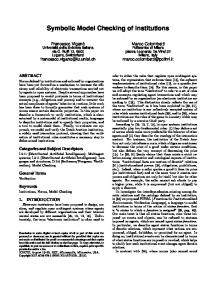
A.5 Demonstration A.5.1 Specification Editor: Fig. 3 shows the specification editor which is used to specify the model and the verified properties. Another way to define a process in PAT is to draw the process as a finite state machine in the LTS Canvas. Fig. 2 is a different definition of Phil() process.
LTS Canvas
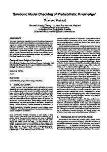
A.5.2 Simulator: We will illustrate the simulator (Fig. 4) using the previous loaded example. Firstly, we will show the complete states graph generated based on the execution. Secondly, we will play the animation of automatically random simulation. Thirdly, we will show how the user guided simulation is conducted step-by-step. Finally, we will demonstrate the functions of execution trace display and replay. A.5.3 Verification: We will verify properties in the Dining Philosopher example to illustrate the verification support (see Fig. 5). A.6 Experiments Table I summarizes the comparison on benchmark systems in terms of the number of Boolean variables (#Var), maximum size of the BDD during verification (S), and verification time (T). The test bed is a PC with Intel Core 2 Duo E6550 CPU at 2.33GHz and 3GB RAM. In the sample systems, the hierarchy of systems are measured by the number of composition operators (e.g. parallel composition and non-deterministic choice) used to compose the system. According the extent of the hierarchy, these examples can be divided in 2 groups. The first group contains systems composed of a few complex primitive components (module in NuSMV). The second group includes systems composed of a number of simple primitive components. A.7 Conclusion and Future Works In the end, we would like to briefly talk about the related work and future research directions.
Figure 3.
Main Window of LTS module with Dining Philosopher example
Figure 4.
Process Simulation Screen
Figure 5.
Verification Panel