IAPR TECHNICAL PAPER SERIES
LEVELS OF DISAGGREGATION AND DEGREES OF AGGREGATE CONSTRAINT IN TRANSPORTATION SYSTEM MODELING J.D. Hunt Department of Civil Engineering and Institute for Advanced Policy Research University of Calgary
October 2006
Technical Paper No. TP-06016
Institute for Advanced Policy Research University of Calgary Calgary, Alberta Canada
http://www.iapr.ca
[email protected]
@ by author. All rights reserved. Short sections of text, not to exceed two paragraphs, may be quoted without explicit permission provided that full credit is given to the source. Correspondence: J.D. Hunt,
[email protected]
Levels of Disaggregation and Degrees of Aggregate Constraint in Transportation System Modeling JD Hunt Professor of Transportation Engineering and Planning Department of Civil Engineering, Schulich School of Engineering Institute for Advanced Policy Research University of Calgary Email:
[email protected] For consideration for publication in Transport Reviews journal Calgary AB, Canada October 2006
Abstract This paper considers the range of different approaches used in the modeling of transportation systems and urban systems more generally. It does so in terms of two dimensions: (a) the level of disaggregation in the representation of system elements and (b) the degree of aggregate constraint on the model system. A range of points or regions are defined along each of these dimensions, including the ‘equilibrium’ and the ‘process simulation’ approaches as two alternatives along the second dimension. Specific modeling approaches are located within the 2-dimensional continuum defined by these two dimensions, including traditional and newly emerging approaches. This provides a framework for (a) discussing the advantages and disadvantages within the range of available techniques and the potential for matching technique with context in a given instance; (b) presenting a more complete view of the linkages among techniques and the scope for hybrid approaches; (c) identifying issues regarding model system dynamics, convergence and the uniqueness of solutions that arise with the practical implementation of transportation system models generally and the latest activity-based models in particular, helping progress beyond the standard positions in the current ‘equilibrium versus process simulation’ debate; and (d) aiding the consideration of appropriate directions for further research and development work. Key Words: transportation modeling approaches; urban system modeling approaches; equilibrium; microsimulation; agent processes; model system iterations and convergence; model system behavior and dynamics
Levels of Disaggregation and Degrees of Aggregate Constraint in Transportation System Modeling JD Hunt File: Disaggregation and Aggregate Constraint.01.TransportReviews.doc Transport Reviews MANUSCRIPT FOR CONSIDERATION Page 2 of 20
Introduction Modeling approaches used in transportation system modeling and in urban system modeling more generally can be considers in terms of two dimensions: (a) the level of disaggregation in the representation of system elements and (b) the degree of aggregate constraint on the model system. The bulk of existing approaches in transportation system modeling tend to sit very broadly along a ‘diagonal’ in these two dimensions running from the ‘aggregate and equilibrium’ combination to the ‘disaggregate and process simulation’ combination, but a range of other approaches including some more novel ones that sit off this diagonal are also available. This paper presents, in order: • Descriptions of the ‘equilibrium’ and the ‘process simulation’ modeling approaches and their properties, outlining the elements of the debate concerning their relative merits and (perceived?) flaws; • Definition of the degree of aggregate constraint on the model system as a dimension along which different types of modeling approach can be placed, including identification of the relevant model system attributes and the further definition of different categories of approach as points or regions along this dimension in terms of these codified system attributes, including the ‘equilibrium’ and the ‘process simulation’ approaches as two such regions; • Definition of the level of disaggregation in the representation of system elements as another such dimension along which different modeling approaches can be placed, again defining specific regions along this dimension. • Consideration of the above two dimensions jointly, defining a continuum on which various specific model systems and approaches are located and regions of emergent and chaotic behavior are identified; • Identification and discussion of the broad ‘diagonal’ trend on this two-dimensional continuum for the range of existing approaches in transportation system modeling, along with consideration of examples of more novel approaches that depart from this diagonal trend; and • Conclusions arising from considerations facilitated with the taxonomy based on these two dimensions and the regions along them. Equilibrium vs Process Simulation It is a standard view in transportation system modeling – almost a central tenet in the orthodoxy – that there are two basic types of modeling approach available: ‘equilibrium’ versus ‘process simulation’. With the equilibrium approach a particular state of the model system with certain properties is identified, a calculation process is used to (iteratively) bring the system to this particular state (sometimes called the ‘equilibrium solution’) and then other aspects of the system at this state are examined and perhaps compared with what they are at the same particular state under other conditions. The standard 4-step model (with feedbacks) uses the equilibrium approach.
Levels of Disaggregation and Degrees of Aggregate Constraint in Transportation System Modeling JD Hunt File: Disaggregation and Aggregate Constraint.01.TransportReviews.doc Transport Reviews MANUSCRIPT FOR CONSIDERATION Page 3 of 20
With the process simulation approach an explicit reproduction of certain elements of the behavior of the real-world system is developed, including representation of the separate actions and reactions involved (and often involving a direct representation of behavior through time). A calculation process is then used to work through the sequence of combined actions that arise under specific initial conditions. Aspects of the model system through this sequence are examined and perhaps compared with what they are through the same sort of sequence under other starting conditions. The activity-based model system and the latest in traffic microsimulation modeling use this approach. Each approach has advantages and disadvantages. For the equilibrium approach: • It considers a well-defined system state that is at least identifiable and in many cases is unique, allowing re-identification and re-examination; • The solution point can have certain properties that allow theoretical extensions or reinterpretation of results, such as socially-desirable allocations of resources in welfare economics analysis (Shoven and Whalley, 1992; Quirk and Saposnik, 1968); pricing strategies and second-best approaches (Lipsey and Lancaster, 1956); non-Walresian or reduced assumptions (Makowski and Ostroy, 1995; Dixit and Norman, 1980); and contestable markets (Brock, 1983); and the ‘all-used-paths-have-same-minimum-cost’ property with transport networks in certain forms of equilibrium (Ortúzar and Willumsen, 1994); • The solution point can have certain properties that make it relatively easy (or quick) to find (such as with the Frank-Wolfe Algorithm (Ortúzar and Willumsen, 1994)); • The defined equilibrium state generally does not exist in reality for most systems of interest except with more generalized and extended (perhaps sometimes even stretched?) definitions of equilibrium, such as spatially or temporally dynamic-equilibrium (Arrow and Debreu, 1954; Grandmont, 1977) that may also give up something with regard to the benefits of the other properties listed above, including the potential instability and non-uniqueness of equilibrium points (Mandler, 1999); and • Failure to reach the defined equilibrium point within a sufficient tolerance can lead to difficulties when interpreting results, particularly when comparing results for different input conditions, leading to the potential for large calculation burdens and such that iteration ‘recipes’ are a poor compromise. For the process simulation approach: • It provides a more direct match with actual system mechanics; • It generally can draw on a wider range of understanding and appreciation of the elements of behavior involved; • It does not require the definition of an equilibrium state or even rely on the concept of equilibrium; • It incorporates path dependencies that complicate understanding and evaluation; • It can display ‘emergent’ aggregate behavior, leading to a greater appreciation of system dynamics; • It typically involves random elements in its calculation processes (using Monte Carlo
Levels of Disaggregation and Degrees of Aggregate Constraint in Transportation System Modeling JD Hunt File: Disaggregation and Aggregate Constraint.01.TransportReviews.doc Transport Reviews MANUSCRIPT FOR CONSIDERATION Page 4 of 20
•
techniques) with the implication that the calculated output values also have random components (sometimes called ‘simulation error’ or ‘microsimulation error’) with distributions that vary with level of aggregation and often are not well understood; and The calculation of expectations for outputs in general requires multiple simulation runs, leading to the potential for large calculation burdens.
Both of these approaches have their proponents, and the debates that arise about the relative merits of the two approaches can sometimes be heated. This is hardly surprising, as these two approaches arise from very different viewpoints and the strength and indeed even the relevance of the advantages and disadvantages vary according to theoretical perspective and modeling context more generally. In essence the equilibrium approach facilitates a more wide-ranging theoretical consideration of the cross-sectional tendencies of the system whereas the process simulation approach allows a more empirical exploration of the actual dynamic behavior of the system. Two misconceptions that often arise (among many potential ones) are: (1) that the iterations used in a calculation process to find the equilibrium solution in some way mimic the real-world behavior of the system, which would be the case only by coincidence; and (2) that the simulation error in some way mimics the variation in system behavior even when the random elements involved in the calculation process reflect analyst uncertainty rather than variation in system behavior, which again would be the case only by coincidence. Degree of Aggregate Constraint The equilibrium approach and the process simulation approach can be characterized as two points (or even regions?) on a continuum regarding the extent that an aggregate state is imposed on the model system – either explicitly at an aggregate level or implicitly via disaggregate elements – when the system is ‘run’. At the one end of this continuum is a complete lack of any aggregate constraints or restrictions on the system and at the other end is a full set of such constraints. A ‘run’ of the model system in this sense is the performance of iterative calculations (almost certainly by computer) in the search for a defined state and/or the working through of the implications of the interactive behavior of the system elements. It involves the determination and transfer among the system elements of various internal ‘signals’ (volumes, demands, prices, etc) that coordinate the responses of the elements, including ‘feedbacks’ impacting the evolution of the system. This iterative evolution of the system during a ‘run’ can be represented using the following general equation: Si + εi = f( Si-1 + εi-1, P, O ) where: i = index representing iterations; = system state at iteration i; Si εi = ‘epsilon ball’ representing variation in system state at iteration i along the full set of dimensions relevant to Si;
Levels of Disaggregation and Degrees of Aggregate Constraint in Transportation System Modeling JD Hunt File: Disaggregation and Aggregate Constraint.01.TransportReviews.doc Transport Reviews MANUSCRIPT FOR CONSIDERATION Page 5 of 20
f(..) P O
= iterative update behavior of system; = vector of model parameters; and = vector of iteration starting conditions.
Different points or regions along the continuum regarding the degree of aggregate constraint on the system can be defined using the components of the above equation, along with the following specific limits regarding these components: S = lim i
→ ∞
Si
and ε = lim i
→ ∞
εi
.
Definitions of potential points or regions that together span this continuum are set out below. Aggregate System Optimal At one end of the continuum regarding the degree of aggregate constraint is the ‘aggregate system optimal’ category of approach, where the defining characteristic is the application of a strong constraint requiring the identification of the unique system state where some aggregate measure of the system is optimized. In terms of the above equation elements, S is unique, ε is 0, O has no impact on S and some function k(S) is maximized or minimized at k(S). Examples of the use of this approach are: • models based on the minimum total cost mathematical programming setup, such as POLIS (Caindec and Prastacos, 1995; Prastacos, 1986a;b) and various models by Boyce (1988), Boyce et al (1987; 1983) and Kim (1979); • normative planning models, such as TOPAZ (Brotchie et al, 1980) nd • Wardrop’s 2 Equilibrium or ‘Social Equilibrium’ in traffic network assignment (Wardrop, 1952). An essential element of this category of approach is the existence of a unique S with the required property regarding k(S) for the system. If there are multiple S with this property, or the search process (the f(..) identified above) is only certain to locate a local rather than a global maximum or minimum for k(S), then the approach falls into a category of approach with a weaker level of aggregate constraint called the ‘converged’ category, which is discussed further below. Particular instances of the ‘aggregate system optimal’ approach can also display the defining characteristic of the ‘equilibrium’ category of approach – that some disaggregate component or components of the system are optimized at S, as is discussed further below. Wardrop’s 2nd Equilibrium is one such approach. These approaches and/or their results are sometimes referred to as ‘strong equilibrium’ in recognition of this additional property.
Levels of Disaggregation and Degrees of Aggregate Constraint in Transportation System Modeling JD Hunt File: Disaggregation and Aggregate Constraint.01.TransportReviews.doc Transport Reviews MANUSCRIPT FOR CONSIDERATION Page 6 of 20
Equilibrium Moving away from the end of the continuum occupied by the ‘aggregate system optimal’ category of approach involves removing the requirement that an aggregate measure concerning the entire system is optimized at the solution point and replacing it with the slightly weaker requirement that one or more measures concerning just sub-components of the system are optimized. The category of approach in this ‘broader’ region is the ‘equilibrium’ category. In terms of the above equation elements, the defining characteristics of the ‘equilibrium’ category are that S is unique, ε is 0, O has no impact on S and some function or functions mn(S) are maximized or minimized at S. Examples of the use of this approach are: • transportation planning forecasting models using the 4-step process with full feedbacks, such as the Edmonton Transportation Analysis Model (Hunt, 2003a; Hunt et al, 1998); • land use transport interaction models using the MEPLAN (Hunt and Simmonds, 1993) or TRANUS (de la Barra et al, 1984; Modelistica, 1995) frameworks; st • Wardrop’s 1 Equilibrium or ‘User Equilibrium’ in traffic network assignment (Wardrop, 1952); and • Nash Equilibrium (Nash, 1950). Again, an essential element of this category of approach is the existence of a unique S with the required properties regarding the mn(S) for the system. The existence of multiple S with this property, or uncertainty about the ability of the applied search process to locate global rather than local maxima or minima for the mn(S), moves the approach to the ‘converged’ category. As indicated above, instances of the ‘equilibrium approach’ can also display the defining characteristic of the ‘aggregate system optimal’ category – but they do not have to. Wardrop’s 1st Equilibrium is an example of an approach where the mn(S) is optimized but the k(S) in general is not optimized at S. In such cases, the approach and/or its results are sometimes referred to as ‘weak equilibrium’. Agent Processes At the opposite end of the continuum is the ‘agent processes’ category of approach, where the defining characteristic is the lack of any effective or specific constraints on the aggregate system behavior. Any patterns in aggregate behavior that do arise are solely ‘emergent’ from the working through of the implications of the interactive behavior of the disaggregate system elements. In terms of the above equation elements, S and ε are fully random, emergent without external constraint and unbounded in the range of variation, and O has a large role in influencing the central tendencies of both S and ε. Examples of the use of this approach are: • SWARM models (Minar et al, 1996); • Brownian Motion Models of gases (Harrison, 1986); and • Models of moving flocks of birds and herds of animals (Reynolds, 1987). In general, it will be possible to describe the variations in S and ε arising with such approaches
Levels of Disaggregation and Degrees of Aggregate Constraint in Transportation System Modeling JD Hunt File: Disaggregation and Aggregate Constraint.01.TransportReviews.doc Transport Reviews MANUSCRIPT FOR CONSIDERATION Page 7 of 20
using statistical distributions, perhaps even parametric distributions. But in the context of the discussions here this amounts to the fitting of such distributions ex post, as a description of the pattern of the emergent results, not the application of a statistical model at an aggregate level in the generation of the results. In this sense, the Central Limit Theorem, and other similar closed-form demonstrations of the inevitable patterns arising in aggregate as a result of the conditions under which the disaggregate elements are acting and interacting, are viewed as more general descriptions of how disaggregate actions and interactions give rise to an aggregate pattern – an aggregate pattern that is ‘emergent’ in the context of this work. The model system in this context is representing not only the aggregate pattern, but also the disaggregate behavior giving rise to that pattern, and doing so according to rules expressed at the disaggregate level. The essential element here – that distinguishes this category of approach from others considered below – is fully random and unbounded nature of the variations in S and ε that arise. To the extent that explicit bounds are placed on the variations in S and ε – either more ‘gently’ via the nature of the rules governing the behavior of the disaggregate elements or more ‘firmly’ via the imposition of direct constraints at the aggregate level – the modeling approach moves away from this end of the continuum. Chaotic Systems Moving away from the end of the continuum occupied by the ‘agent processes’ category of approach involves acknowledging the ‘most gentle’ influence on the variation in aggregate results arising with the explicit rules governing the behavior of the disaggregate elements of the system, where the system in aggregate displays chaotic behavior, rather than random behavior, and S acts as a strange attractor. O has a large impact on S to the extent that it influences the strange attractor properties of S. Examples of the use of this approach are: • Models of simple mechanical systems, see for example Kapitaniak (1988); and • Fractal repetitive systems – such as Mandelbrot drawings (Mandelbrot and Wheeler, 1983). The switch in S from a random variable to a strange attractor – that moves the approach from the ‘agent processes’ category to the ‘chaotic system’ category – occurs entirely as a result of changes in the representation of the behavior of the disaggregate elements of the system. A minor level of aggregate constraint is being imposed with the move to the ‘chaotic system’ category, but in a ‘most gentle’ manner via the disaggregate elements. Stable Bounded Continuing in the move away from the ‘agent processes’ end of the continuum, the next category of approach after ‘chaotic systems’ is ‘stable bounded’. The defining characteristic of the ‘stable bounded’ category of approach is that S and ε vary within a bounded range, possibly following a repeating pattern within that range and with the boundary limits influenced or even imposed by O. Examples of the use of this approach are: • Many of the models of competing biological populations over time and/or space (Hofbauer
Levels of Disaggregation and Degrees of Aggregate Constraint in Transportation System Modeling JD Hunt File: Disaggregation and Aggregate Constraint.01.TransportReviews.doc Transport Reviews MANUSCRIPT FOR CONSIDERATION Page 8 of 20
•
and Sigmund, 1998; Amarasekare and Nisbet, 2001; Coste et al, 1979), with the proviso that these models can sometimes fall into the ‘chaotic systems’ category; and Some traffic assignment algorithms with ‘hard speed changes’ such that the update signal from one iteration to the next is not damped sufficiently and the process jumps between solution points without converging (Ortúzar and Willumsen, 1994)
The imposition of the boundary limits on the variation in S and ε may occur either more ‘gently’ via the representation of the behavior of the disaggregate elements of the system (as is the case with the ‘chaotic system’ category of approach) or more ‘firmly’ via the direct imposition of aggregate rules. Converged Moving further along the continuum in the direction of increasing aggregate constraint, the next category after ‘stable bounded’ is the ‘converged’ category of approach, where the solution space is a set of multiple, non-unique points. Specifically, there is a vector of multiple and separate S, ε is 0, and O has an impact on the particular separate point that is S in a given instance. Approaches fall into this category when there are multiple system states that satisfy the criteria defining the solution, when the search process (the f(..) identified above) is unable to discern a local from a global optimum regarding its search criteria or when the system has inherent path dependences. In the first and second of these cases, the existence of multiple and separate S may be the unintended consequence of an inadequately specified solution or inadequately designed search process, not an essential (or even anticipated) property of the corresponding real-world system being modelled. In the last of these cases, multiple and separate S are an essential aspect of the system. Examples of the use of this approach are: • Iterative proportional fitting processes, including Fratar (1954) and Furness (1970) matrix adjustment procedures, where O is taken to be the seed matrix or the initial set of covariances among the matrix dimensions; • Population synthesis processes where objects are drawn from a pool and accepted consistent with specified marginal distributions on various attributes of the objects in aggregate (Beckman et al, 1996); • Search processes where the number of iterations is limited to a specified maximum, including so-called ‘iteration recipes’, where O is taken to include the value of this specified maximum; • Some forms of urban system models allowing polycentric forms (Anas and Kim, 1996); and • Method of Successive Averages (MSA) used in traffic network assignment (Ortúzar and Willumsen, 1994). Path Independence The ‘path independence’ category of approach is located along the continuum between the ‘converged’ and the ‘equilibrium’ categories, where there is only one solution found by the search process, regardless of the starting point for the search, and this point is defined in terms of some form of search rule that does not relate to the optimization of either an aggregate measure
Levels of Disaggregation and Degrees of Aggregate Constraint in Transportation System Modeling JD Hunt File: Disaggregation and Aggregate Constraint.01.TransportReviews.doc Transport Reviews MANUSCRIPT FOR CONSIDERATION Page 9 of 20
concerning the entire system or any measures concerning sub-components of the system. In terms of the equation elements, S is unique, ε is 0, and O has no impact on S. This is similar to the ‘equilibrium’ category, but without any function or functions mn(S) that are maximized or minimized at mn(S) and thus without the associated equilibrium interpretation regarding the solution. Examples of the use of this approach are: • Markov chain models (Markov, 1971); and • SATURN (Van Vliet, 1982) and CONTRAM (Taylor, 2003) models (possibly), where the origin-destination matrix of vehicle demands is fixed and not considered part of O It seems likely that certain forms of iteration recipe for f(..) can be expected to work to identify unique and stable solutions that do not necessarily maximize or minimize any function mn(S) – in particular when the recipe considers only the magnitude of the change from Si-1 to Si, and its implication for ε, when determining whether to stop and declare that convergence has been achieved and thus S has been found. In such cases the approach falls into the ‘path independence’ category. In some cases it may be difficult to discern if a given approach belongs in the ‘equilibrium’ category or the ‘path independence’ category – because it may be difficult to say if the solution has an appropriate equilibrium interpretation. That is, there may be one or more functions mn(S) that are maximized or minimized at S such that an equilibrium interpretation of the solution is available and could be applied – if the definition of equilibrium is extended (or even tortured?) sufficiently. In this regard it should be noted that there is an entire vein of ongoing work seeking to extend the definition of equilibrium and also cast the range of steady state conditions for dynamic systems in terms of equilibrium concepts in order to unite the two areas where possible; see for examples Boulding (1956), Cantarella and Cascetta (1995), Ye et al (1998) and Wiggins (2003). The implication is that many ‘path independence’ approaches can perhaps be moved to a broader ‘equilibrium’ category provided there is enough stretching of the definition of equilibrium. It is sufficient in this discussion to note that the boundary between these two categories is dependent on the definition of equilibrium – and that as the definition of equilibrium is expanded so is the ‘equilibrium’ category of approach expanded. Together, these different categories of approach regarding the degree and nature of aggregate constraint on the model system cover the full range of treatments applied in the representation of aggregate system behavior. As such, they provide a classification system regarding the aggregate behavioral construct being used. Specific modeling approaches can be placed along this continuum, referring to the nature of the constraints being enforced and the aggregate behavioral construct being applied as a result. Level of Disaggregation There is another continuum along which categories of approach can be defined, one that is related to the continuum regarding the degree of aggregate constraint considered above. This other continuum concerns the level of representation of the individual behavioral agents in the system and the distributions of their interactions. It ranges from the explicit treatment of each agent as a unique
Levels of Disaggregation and Degrees of Aggregate Constraint in Transportation System Modeling JD Hunt File: Disaggregation and Aggregate Constraint.01.TransportReviews.doc Transport Reviews MANUSCRIPT FOR CONSIDERATION Page 10 of 20
object to the handling of aggregate quantities representing groups or flows of agents as specific entities. Definitions of potential points or regions that together span this continuum regarding the behavioral unit are set out below. Entire Aggregate Population The ‘entire aggregate population’ category of approach is at one end of the continuum regarding the level of representation of the individual behavioral agents, where there is one, all-inclusive quantity used to represent the entire population of agents. It is the behavior of this entire population that is represented explicitly, as a quantity or flow that responds to system-wide inputs and signals directly. Examples of the use of this approach are: • Direct-demand models (Ortúzar and Willumsen, 1994), also called ‘simultaneous’ models, with specific examples by Asri and Sugie (2003) and Quandt and Baumol (1966); • Supply curves on their own and demand curve on their own in Classical Economics; Note that representations of market behavior using supply curves and demand curves interacting together fall into the ‘aggregate population segments’ approach as defined below because of the consideration of supply and demand as two segments; and • Simple single-point representations of systems, as is done in the representation of location trajectories and in the development of Mandelbrot drawings (Mandelbrot and Wheeler, 1983). Aggregate Population Segments Moving away from the end of the continuum occupied by the ‘entire aggregate population’ category of approach involves separating the single category representation of the entire population of agents into two or more segments. The explicit representation concerns the behaviors of these segments and their interactions, again, as quantities or flows where each such quantity or flow directly responds to signals and perhaps also provides signals. The resulting overall behavior of the system arises as a result of the interactions among the constituent quantities or flows responding directly as represented, with the ‘run’ of the model system being the working through of the implications of the interactive behavior of the various aggregate segments. Examples of the use of this approach are: • Representations of market behavior in classical economics using supply curves and demand curves interacting together; • Aggregate steady-state traffic assignment, with the flow for each origin-destination pair constituting a different segment, and any segmentation with multi-class assignment; and • Aggregate 4-step (or, more broadly, n-step) transportation planning models. In the most general sense, the definition of this category can be ‘stretched’ to include the special case where there is a single agent in each segment in the model and the explicitly represented behavior of the segment in each instance is actually the behavior of the single agent in the segment – such that the explicit representation of behavior in effect concerns the behavior of agents rather than
Levels of Disaggregation and Degrees of Aggregate Constraint in Transportation System Modeling JD Hunt File: Disaggregation and Aggregate Constraint.01.TransportReviews.doc Transport Reviews MANUSCRIPT FOR CONSIDERATION Page 11 of 20
the behavior of groups or flows of agents. Two forms of this special case can be identified: • Where there are as many model segments as there are agents in the real-world system being represented; and • Where there are fewer model segments than there are agents in the real-world system being represented, and the model representations for some segments correspond to groups of more than single agents in the real-world system. In this discussion, these two forms of this special case are considered to be separate categories (which are defined below) and the range of the ‘aggregate population segments’ category considered here is defined to include only those cases where there is more than one agent in each model segment. The essential element is that the explicit representation of behavior for a segment concerns the behavior of a group of more than one agent – when this is the case, the approach falls into the ‘aggregate population segments’ category. For completeness, in this context, cases where some model segments include just one agent and other model segment include multiple numbers of agents are considered to constitute mixed approaches involving the different categories to the extent they are represented. Sample Enumeration Continuing in the move away from the ‘entire aggregate population’ end of the continuum, the next category of approach after ‘aggregate population segments’ is ‘sample enumeration’. In the ‘sample enumeration’ approach, the behavior of each of a set of individual agents is represented explicitly and the results for each of these modeled agents are multiplied, or ‘expanded’, to establish the results for the portion of the real-world population of agents represented by the modeled agent. The results thus established for the different portions of the real-world population are then combined to establish the results for the full real-world population. This ‘sample enumeration’ category is one of the forms of special case identified above – the one where there is a single agent in each segment in the model and where there are fewer model segments than there are agents in the real-world system being represented such that the model representations for some segments correspond to groups of more than single agents in the real-world system. Examples of the use of this approach include: • The SATURN (Van Vliet, 1982) and CONTRAM (Taylor, 2003) traffic assignment procedures, where packets of multiple numbers of vehicles are routed through networks; and • Some specialized travel demand forecasting systems, including ones developed using the Apply functionality available in the ALOGIT software (Daly, 1992) such as the Channel Tunnel Rail Link (Hague Consulting Group, 1995) and the Oresund Fixed Link forecasting tools (Daly et al, 1999). The key elements defining this category of approach are (a) the explicit representation of behavior at the level of the individual model agent and (b) the expansion of the results for individual model agents to establish the results for the corresponding aggregate groups of real-world agents. This mix of direct treatment of both individual agents and aggregate groups of agents places the ‘sample enumeration’ category of approach in the middle-ground of the continuum concerning level of
Levels of Disaggregation and Degrees of Aggregate Constraint in Transportation System Modeling JD Hunt File: Disaggregation and Aggregate Constraint.01.TransportReviews.doc Transport Reviews MANUSCRIPT FOR CONSIDERATION Page 12 of 20
representation. Observed Agents The ‘observed agents’ category of approach is at the opposite end of the continuum from the ‘entire aggregate population’ end. It uses the most disaggregate representation possible, where there is a one-to-one correspondence between agents in the real world and agents in the model and the model provides explicit representation of the behavior of these corresponding agents. The explicit representation of behavior in the model does not have to be a perfect description of actual behavior (realistically, how could it be?), it merely has to concern an individual model agent in each case where this model agent corresponds one-to-one with a specific real-world agent. In addition, with the ‘observed agents’ category of approach, the description of each agent in the model is based on observation of the corresponding real-world agent – which means that the description of the agent is also as specific as possible. This is in contrast to the description of each agent being developed synthetically, which is what characterizes the ‘synthetic agents’ category of approach defined below. Examples of the use of the ‘observed agents’ category of approach include: • PECAS-SD (Hunt et al, 2004) and UrbanSim (Waddell, 2002) land development models, at least by intention and to the extent that synthesis of land attributes is avoided; and • UPlan (Johnston and Shabazian, 2003) land use allocation system. Synthesized Agents Moving back a bit from the ‘observed agents’ end of the continuum, the next category of approach is ‘synthesized agents’. The ‘synthesized agents’ category of approach is like the ‘observed agents’ category in that there is a one-to-one correspondence between agents in the real world and agents in the model and the model provides explicit representation of the behavior of these corresponding agents. But, as indicated above, with the ‘synthesized agents’ category of approach the description of each agent is developed synthetically, perhaps using some form of random draws from relevant sampling distributions in order to establish the states for the vector of attributes describing each agent, as is done with population synthesis processes (Beckman et al, 1996). The bulk of the current work on activity-based and tour-based travel microsimulation and on traffic microsimulation falls within this category of approach, including, for example: • San Francisco SFCTA model (Jonnalagadda et al, 2001); • MORPC model (Bradley and Vovsha, 2005); and • Fully dynamic traffic microsimulations, such as PARAMICS (SAIS, 1999) and VISSIM (PTV, 2003). Degree of Aggregate Constraint and Level of Disaggregation Together Specific modeling approaches can be placed along these two continua jointly in a 2-dimensional plane. This is done in Figure 1 for a selection of modeling approaches.
Levels of Disaggregation and Degrees of Aggregate Constraint in Transportation System Modeling JD Hunt File: Disaggregation and Aggregate Constraint.01.TransportReviews.doc Transport Reviews MANUSCRIPT FOR CONSIDERATION Page 13 of 20
direct demand models
entire aggregate population
supply-demand curves Wardrop 2nd
Wardrop 1st
MSA
multi-class assignment TOPAZ POLIS
Furness
competing biological population simulations
MEPLAN, TRANUS LOWRY, PECAS-AA
sample enumeration
SATURN CONTRAM
emergent
SWARM
Oregon2 synthesized agents
SOLUTIONS
observed agents
simulated annealing Paramics population synthesis VISSIM activity-based travel demand Calgary CVM UPlan
aggregate system optimal
equilibrium
Mandelbrot drawings
simple mechanical systems
Frank-Wolfe
aggregate population segments behavioural unit
chaotic
path independence
converged
ALBATROSS BE-microsim PECAS-SD UrbanSIM Land ILUTE
stable bounded
agent processes
degree of aggregate constraint
Figure 1: Comparison of modeling approaches concerning level of aggregation (the behavioral unit) and degree of aggregate constraint (the aggregate behavioral construct). Figure 1 also shows regions with chaotic and/or emergent aggregate behavior. This is based on a recognition that chaotic behavior tends to arise when there are comparatively fewer agents – consistent with the idea that a larger number of individual objects with a comparatively wide distribution of responses results in a dissipation of impact that dampens the system. This is also based on the recognition that emergent aggregate behavior only arises in a meaningful sense when there are enough individual agents to allow for the interactions among these agents to develop into something beyond what is specified explicitly among these agents. A Taxonomy of Transportation System Modeling Approaches The existing approaches in transportation system modeling tend to sit along a diagonal from upperleft to lower-right in Figure 1; the recent increasing use of process simulation has arisen in conjunction with a swing to greater use of explicit representation of individual agents. Clearly, the ability to handle systems with large numbers of interacting agents (with the advent of increasing computing capabilities) has led to more attempts at explicit representation of the behavioral processes involved at the individual level. It would appear that more and more analysts are taking the view – at least implicitly – that enough is known about the nature of the behavior of the individual agents involved (possibly in part because these analysts are such agents themselves in the
Levels of Disaggregation and Degrees of Aggregate Constraint in Transportation System Modeling JD Hunt File: Disaggregation and Aggregate Constraint.01.TransportReviews.doc Transport Reviews MANUSCRIPT FOR CONSIDERATION Page 14 of 20
real world and thus have insight gained by experience) to result in model systems that provide more accurate – or at least more faithful – representations of reality. One of the points to be made here is that a range of other combinations off the diagonal are available in transportation system and related modeling. Some of these other combinations are now being explored in order to gain some of the advantages that are available. Examples of these other combinations are: (a) Cambridge SOLUTIONS model system (Caruso, 2005): This uses a bid-choice framework to allocate individual households to residential locations within a particular transportation analysis zone consistent with the results of an equilibrium-based combined land use transport model (using the MEPLAN framework) in order to refine the search for the equilibrium solution and further explore the aspects of this equilibrium solution at the level of individual households. A detailed resolution is provided without giving up desirable equilibrium properties. (b) Calgary Commercial Vehicle Movements Model (CVM) (Stefan et al, 2005): This uses a tour-based microsimulation framework with Monte Carlo simulation where logit choice models provide the sampling distributions in order to simulate the movements of commercial vehicles in the delivery of goods and services. It runs in combination with an equilibrium-based model of household travel demands. Trip tables from multiple runs of the commercial movement model are averaged in order to obtain a trip table of expected movements, and this is combined with trip tables from the households demands model and then assigned to road networks using stochastic user equilibrium techniques. The resulting congested travel times are fed back to both the households demands model and the commercial vehicle movements model in an iterative process that runs to a convergence. A converged system is obtained with a household demand model at equilibrium and a process simulation tour-based microsimulation representation of commercial vehicle movements. (c) Oregon2 Integrated Land Use Transport Model (Hunt, 2003b; Hunt et al, 2001): This includes a spatially disaggregated input-output model based on equilibrium to represent industrial and government activity and process-oriented microsimulations of household demographics and travel activities (activity-based) and land development activity, with the interface between these occurring at the represented markets, where elasticities in the provision of labor by workers and in the use of developed space by activities allow for consistent market-clearing to occur. The situation with activity-based models is likely to warrant similar combined treatments in some instances, where an assignment process is used to identify an equilibrium state for the network between supply and demand. Expectations of the quantities of household travel demand are the quantities being loaded to the network, with these developed using an activity-based model component run multiple times within each iteration of the assignment process. Using the definitions established above, such a combined treatment would constitute less of a process simulation and more of a disaggregation of the household demand side of the network equilibrium. To date there has been little in the literature about the issues arising with such a combined treatment; at the least it should be acknowledged that there is still a ‘reliance’ on the concept of equilibrium even with an
Levels of Disaggregation and Degrees of Aggregate Constraint in Transportation System Modeling JD Hunt File: Disaggregation and Aggregate Constraint.01.TransportReviews.doc Transport Reviews MANUSCRIPT FOR CONSIDERATION Page 15 of 20
activity-based model being used. Discussion The ‘equilibrium’ and ‘process simulation’ techniques both sit in a larger continuum involving the degree of aggregate constraint on the model system; and combined techniques involving elements of both are being used in practice. It seems likely that practical applications of activity-based models will often involve such combined techniques. Certainly, the use of an activity-based approach does not preclude the use of equilibrium techniques, and there indeed may be good reasons for the two to be used in combination. The practical implementation of model systems using combinations of process simulation and equilibrium techniques underway at present is being guided largely by intuition and some potentially relevant previous experience. There is little that is understood from a more general theoretical perspective. Some more generalized theoretical research needs to be done considering the issues involved, including: • the uniqueness of converged solutions; • the extent that equilibrium properties apply; • the possible combinations and variations in techniques and the advantages and disadvantages arising with each; • the relevant attributes to use in the definitions of the relevant categories properties; and • the potential linkages among the ‘strange attractors’ in chaotic systems. The results of this more generalized theoretical research then need to be converted into appropriate guidance for practical modeling work. Practice is moving ahead with activity-based modeling (although perhaps not as fast as some would like) and theory needs to catch-up. In this light, the ‘equilibrium versus process simulation’ debate seems mis-directed, and effort should be focused on establishing how to gain the benefits available with each and how to use the two in combination most appropriately. Conclusions In model systems, the level of disaggregation and the degree of aggregate constraint are two different and separable characteristics. It is useful to separate the two when considering the properties of these systems, as it can help in the understanding of the model system dynamics and in the identification of alternative and more suitable modeling approaches and the aspects of the solutions provided by these approaches. Much of the practical work in transportation system modeling tends to sit very broadly along a ‘diagonal’ in these two dimensions running from the ‘aggregate and equilibrium’ combination to the ‘disaggregate and process simulation’ combination. A range of other approaches including some more novel ones that sit off this diagonal are also available, and examples of their use in practical work are now available. One such example is the Cambridge SOLUTIONS model system, where an equilibrium approach is being used in combination with a representation of individual agents at
Levels of Disaggregation and Degrees of Aggregate Constraint in Transportation System Modeling JD Hunt File: Disaggregation and Aggregate Constraint.01.TransportReviews.doc Transport Reviews MANUSCRIPT FOR CONSIDERATION Page 16 of 20
the disaggregate level. The transportation modeling community needs to evolve beyond the ‘equilibrium versus process simulation’ debate. Both have their advantages and disadvantages, and comparative suitability in different contexts. A far more useful and perhaps more challenging pursuit is the design and development of appropriate systems for using the two approaches in combination and an exploration of the relevant properties involving the degree of aggregate constraint dimension identified here. Both theory and practice would benefit from a more generalized theoretical examination of the issues involved, including: (a) the uniqueness of converged solutions; (b) the extent that equilibrium properties apply; (c) the possible combinations and variations in techniques and the advantages and disadvantages arising with each; (d) the relevant attributes to use in the definitions of the relevant categories properties; and (e) the potential linkages among the ‘strange attractors’ in chaotic systems, the converged solutions with equilibrium techniques and the emergent aggregate behavior arising with different sorts of large-scale microsimulations. The definitions provided here, and the resulting taxonomy for sorting model systems along relevant dimensions, is intended as a starting point for such an examination. The issue of the degree of aggregate constraint on the model system needs to be taken into account more completely in much of the current practical work using activity-based models. The focus in such work often seems to be the complexity of the representation of the behavior of the individual agents. Certainly, this aspect of the model is important. But the behavior of the model system in terms of the degree of aggregate constraint is equally important. Practice is moving ahead with activity-based modeling (although perhaps not as fast as some would like) and theory needs to catch-up and provide some important support. The region definitions presented here along the two dimensions are intended to illustrate the range and potential resolution of model system properties. While it is judged that they provide mutually exclusive and collectively exhaustive coverage, they are not intended to be the final, definitive definitions. It certainly may be the case that somewhat different groupings and distinctions would be more appropriate in a given instance and thus it would make sense to modify the ones presented here. Acknowledgements The preparation of this paper was been supported in part by a grant from the National Science and Engineering Research Council of Canada and by the Institute for Advanced Policy Research at the University of Calgary.
References Anas, A. and Kim, I. (1996) General equilibrium models of polycentric urban land use with endogenous congestion and job agglomeration. Journal of Urban Economics 40:232-256.
Levels of Disaggregation and Degrees of Aggregate Constraint in Transportation System Modeling JD Hunt File: Disaggregation and Aggregate Constraint.01.TransportReviews.doc Transport Reviews MANUSCRIPT FOR CONSIDERATION Page 17 of 20
Arrow, K. J. and Debreu, G. (1954). The existence of an equilibrium for a competitive economy. Econometrica 22:265-290. Amarasekare, P. and Nisbet, R.M. (2001) Spatial heterogeneity, source-sink dynamics, and the local coexistence of competing species. The American Naturalist 158:572-584. Boulding, K.E. (1956) General Systems Theory – The skeleton of science. Management Science 2(3):197-208. Boyce, D.E. (1988) Network equilibrium models of urban location and travel choices. a new research agenda. Chapter 14 in New Frontiers in Regional Science: Essays in Honor of Walter Isard, Volume 1. Chatterji, M. and Kuenne, R.E. (Eds.): 238-255. New York University Press, New York. Boyce, D.E, and Lundqvist, L. (1987) Network equilibrium models of urban location and travel choices. Alternative formulations for the Stockholm region. Papers of the Regional Science Association 61:93-104 Boyce, D.E., Chon, K.S., Lee, Y.J., Lin, K.T., LeBlanc, L.J. (1983) Implementation and computational issues for combined models of location, destination, mode, and route choice. Environment and Planning 15A:1219-1230. Bradley, M. and Vovsha, P. (2005) A model for joint choice of daily activity pattern types of household members. Transportation 32:545-571. Brock, W.A. (1983) Contestable markets and the theory of industry structure: a review article. Journal of Political Economy 91(6):1055-1066. Brotchie, J.F., Dickey, J.W. and Sharpe, R. (1980) TOPAZ Planning Techniques and Applications. Lecture Notes in Economics and Mathematical Systems Series. Vol 180. SpringerVerlag, Berlin, Germany. Caindec, E.K. and Prastacos, P. (1995) A Description of POLIS. The Projective Optimization Land Use Information System. Working Paper 95-1. Association of Bay Area Governments, Oakland CA. Cantarella, G.E. and Cascetta, E. (1995) Dynamic processes and equilibrium in transportation networks: towards and unifying theory. Transportation Science 25A(4):305-329. Caruso, G. (2005) SOLUTIONS Micro-Scale Modeling: Method and Initial Results; Draft Working Paper, The Martin Centre for Land Use and Built Form Studies, University of Cambridge, Cambridge, UK. Available on the SOLUTIONS Project Website: http://www.suburbansolutions.ac.uk Coste, J., Peyraud, J. and Coullet, P. (1979) Asymptotic behaviors in the dynamics of competing species. SIAM Journal on Applied Mathematics 36(3):516-543.
Levels of Disaggregation and Degrees of Aggregate Constraint in Transportation System Modeling JD Hunt File: Disaggregation and Aggregate Constraint.01.TransportReviews.doc Transport Reviews MANUSCRIPT FOR CONSIDERATION Page 18 of 20
Daly, A.J. (1992) ALOGIT Users' Guide, Version 3.2: September 1992. Hague Consulting Group, The Hague, The Netherlands. Daly, A.J., Rohr, C. and Jovicic, G. (1999) Application of models based on stated and revealed preference data for forecasting passenger traffic between East and West Denmark. Selected Proceedings of the 8th World Conference on Transport Research 3:121-134. de la Barra, T., Perez, B. and Vera, N. (1984) TRANUS-J: Putting large models into small computers. Environment and Planning 11B:87-101. Dixit, A. and Norman, V. (1980) Theory of Interational Trade: A Dual, General Equilibrium Approach. Cambridge University Press, Cambridge, UK. Fratar, T.S. (1954) Vehicular trip distribution by successive approximation. Traffic Quarterly 8:53-56. Furness, K.P. (1970) Time function interaction. Traffic Engineering and Control 7(7):19-36. Grandmont, J.M. (1977) Temporary general equilibrium theory. Econometrica 45:535-572. Hague Consulting Group (1995) Demand Forecasting for Inter-Urban Traffic on Channel Tunnel Rail Link. Prepared for Union Railways, British Rail Board. Hague Consulting Group, Cambridge, UK. Harrison, J.M. (1986) Brownian motion and stochastic flow systems. Applied Optics 25(18):3145. Hofbauer, J. and Sigmund, K. (1998) Evolutionary Games and Population Dynamics. Cambridge University Press, Cambridge, UK. Hunt, J.D. (2003a) Modeling transportation policy impacts on mobility benefits and KyotoProtocol-related emissions. Built Environment. 29(1):48-65. Hunt, J.D. (2003b) Agent behavior issues arising with urban system micro-simulation. European Journal of Transport Infrastructure and Research 2(3/4):233-254. Hunt, J.D., Abraham, J.E. and T.J. Weidner, T.J. (2004) Land Development Module of the Oregon Framework. Poster presented at the 83rd Transportation Research Board Annual Meeting, Washington DC, USA, January 2004. Hunt, J.D., Donnelly, R.R., Abraham, J.E., Batten, C., Freedman, J., Hicks, J., Costinett, P.J. and Upton, W.J. (2001) Design of a statewide land use transport interaction model for Oregon. Proceedings of the 9th World Conference for Transport Research, Seoul, South Korea, July 2001 (CD-Rom Format).
Levels of Disaggregation and Degrees of Aggregate Constraint in Transportation System Modeling JD Hunt File: Disaggregation and Aggregate Constraint.01.TransportReviews.doc Transport Reviews MANUSCRIPT FOR CONSIDERATION Page 19 of 20
Hunt, J.D., Brownlee, A.T. and Doblanko, L.D. (1998) Design and Calibration of the Edmonton Transportation Analysis Model. Presented at the 1998 Transportation Research Board Conference, Washington DC, USA, January. Hunt, J.D. and Simmonds, D.C. (1993) Theory and application of an integrated land-use and transport modeling framework. Environment and Planning 20B:221-244. Johnston, R. A. and Shabazian, D.R. (2003) UPlan: A Versatile Urban Growth Model for Transportation Planning. Presented at the 82nd Transportation Research Board Annual Meeting, Washington DC, USA, January 2003. Jonnalagadda, N., Freedman, J., Davidson, W.A. and Hunt, J.D. (2001) Development of a microsimulation activity-based model for San Francisco: Destination and mode choice models. Transportation Research Record 1777:25-35. Kapitaniak, T. (1988) Chaos in Systems with Noise. World Scientific, London, UK, 140 pages. Kim, T.J. (1979) Alternative transportation modes in an urban land use model: a general equilibrium approach. Journal of Urban Economics 6:197-215. Lipsey, R.G. and Lancaster, K. (1956) The general theory of second best. Review of Economic Studies 24(1):11-32. Markov, A.A. (1971) Extension of the limit theorems of probability theory to a sum of variables connected in a chain. Reprinted in Appendix B of Howard, R., Dynamic Probabilistic Systems, Volume 1: Markov Chains. John Wiley and Sons, New York NY, USA. Mandelbrot, B.B. and Wheeler, J.A. (1983) The fractal geometry of nature. American Journal of Physics 51:286-287. Minar, N., Burkhart, R., Langton, C. and Askenazi, M. (1996) The SWARM simulation system: A toolkit for building multi-agent simulations. Working Paper 96-06-042, Santa Fe Institute, Santa Fe NM, USA. Mandler, M. (1999) Dilemmas in Economic Theory: Persisting Foundational Problems of Microeconomics. Oxford University Press, Osford, UK. Modelistica (1995) TRANUS Integrated Land Use Transport Modeling System; Version 5.0. Available on the Oregon Department of Transportation Website: http://www.odot.state.or.us Nash, J. (1950) Equilibrium points in n-person games. Proceedings of the National Academy of the USA 36(1):48-49. Ortúzar, JdeD and Willumsen, L.G. (1994) Modeling Transport; Second Edition. Wiley, New York NY, USA.
Levels of Disaggregation and Degrees of Aggregate Constraint in Transportation System Modeling JD Hunt File: Disaggregation and Aggregate Constraint.01.TransportReviews.doc Transport Reviews MANUSCRIPT FOR CONSIDERATION Page 20 of 20
Prastacos, P. (1986a) An integrated land-use-transportation model for the San Francisco Region: 1. Design and mathematical structure. Environment and Planning 18A:307-322. Prastacos, P. (1986b) An integrated land-use-transportation model for the San Francisco Region: 2. Empirical estimation and results. Environment and Planning 18A:511-528. PTV (2003) VISSIM User Manual Version 3.7, PTV AG, Karlsrhue, Germany. Quirk, J.P. and Saposnik, R. (1968) Introduction to General Equilibrium Theory and Welfare Economics. McGraw-Hill, New York NY, USA. Reynolds, C.W. (1987) Flocks, herds and schools: A distributed behavioral model. Proceedings of the 14th Annual Conference on Computer Graphics and Interactive Techniques, ACM Press, New York NY, USA, pp:25-34. SAIS (1999) Paramics User Manual Version 2.2, SIAS, Edinburgh, Scotland. Shoven, J.B. and Whalley, J. (1992) Applying General Equilibrium. Cambridge University Press, Cambridge, UK. Stefan, K.J., McMillan, J.D.P. and Hunt, J.D. (2005) An urban commercial vehicle movement model for Calgary, Alberta, Canada. Transportation Research Record 1921:1-10. Taylor, N.B. (2003) The CONTRAM dynamic traffic assignment model. Networks and Spatial Economics 3:297-322. Van Vliet, D. (1982) SATURN – A modern assignment model. Traffic Engineering and Control 23:578-581. Wiggins, S. (2003) Introduction to Applied Nonlinear Dynamical Systems and Chaos. Texts in Applied Mathematics, Volume 2; 2nd Edition, Springer, New York NY, USA, 808 pages. Waddell, P. (2002) UrbanSim: Modeling urban development for land use, transportation and environmental planning. Journal of the American Planning Association 68(3):297-314. Wardrop, J.G. (1952) Some theoretical aspects of road traffic research. Proceedings, Institute of Civil Engineering, Part II.1:325-378. Ye, H., Michel, A.N. and Hou, L. (1998) Stability theory for hybrid dynamical system. IEEE Transactions on Automatic Control 43(4):461-474.Beckman, R., Baggerly, K. and McKay, M. (1996) Creating synthetic baseline populations. Transportation Research 30A(6):415-435.