A Technique to Calculate Cache Related Preemption ... - Science Direct

Available online at www.sciencedirect.com

ScienceDirect Procedia Computer Science 57 (2015) 622 – 629

A Technique to Calculate Cache Related Preemption Delay using Constraints on Non-Nested Preemptions Ravindra B. Keskar

Umesh Deshpande

Swapnil Kharabe

Department of Computer Science & Engg, Visvesvaraya National Institute of Technology (VNIT), Nagpur, India

Abstract Caches incur an indirect cost to the response times of tasks due to preemptions in a task system. Hence the computation of Cache Related Preemption Delay (CRPD) is an important problem to assess the schedulability of a task system. In this paper, we have introduced the concept of inhibiting and non-nested preemptions. We have proposed a novel method to calculate tight upper and lower bounds on the number of preemptions of every task in the task-system across all phases. The problem of calculation of CRPD is modelled as a constraint satisfaction problem that can be solved by using Integer Linear Programming (ILP). The CRPD values are integrated in the worst case response time analysis. © 2015 The Authors. Published by Elsevier B.V. This is an open access article under the CC BY-NC-ND license (http://creativecommons.org/licenses/by-nc-nd/4.0/).

c 2013 Published by Elsevier of Ltd.  Peer-review under responsibility organizing committee of the 3rd International Conference on Recent Trends in Computing 2015 (ICRTC-2015)

Keywords:

1. Introduction In real time systems, different tasks have timing constraints in terms of deadlines, which the tasks need to meet for a system to be schedulable. In analyzing schedulability of such a system, the cost of task preemption needs to be considered. When a task τi is preempted, many of its blocks in the cache are replaced by the blocks of the preempting task. When τi resumes, the time required for the reloading, called as Cache Related Preemption Delay (CRPD), needs to be considered in the response-time analysis. Many of the methods devised to explicitly calculate the CRPD can be categorized as those considering the effects of the preempting task [1, 2], those considering the effects on the preempted task [3] or both [4, 5, 6]. The framework presented by Lee et al. [4] takes a holistic view to calculate CRPD using constraint-solvers, but the technique is exponential in complexity. Ramprasad and Mueller [5] take into consideration relative phases of the tasks, but require explicit construction of the execution scenario in the hyperperiod. In [6], Staschulat et al. propose an analytical technique to calculate CRPD by independently calculating the number of preemptions and a multiset of possible preemption costs. From the multiset, a number of highest preemption costs are chosen. Work by Altmeyer, Davis and Maiza [7] present different approaches to calculate the preemption cost more accurately by using the multiset technique of Staschulat et.al. [6]. The technique by Lee et.al. [4] tried to explore the solution space by solving a set of constraints using Integer Linear Programming (ILP). The drawback of this method is that the number of terms and the analysis used is exponential. In this work, we present a method for calculation of CRPD costs using ILP that does not have exponential complexity. This is done by using a new concept called as non-nested preemptions. The contributions of this paper are as follows. We define non-nested preemptions (NNP) by introducing a class of preemptions called as inhibiting preemptions. We present a technique that systematically removes the number of

1877-0509 © 2015 The Authors. Published by Elsevier B.V. This is an open access article under the CC BY-NC-ND license (http://creativecommons.org/licenses/by-nc-nd/4.0/). Peer-review under responsibility of organizing committee of the 3rd International Conference on Recent Trends in Computing 2015 (ICRTC-2015) doi:10.1016/j.procs.2015.07.421

623

Ravindra B. Keskar et al. / Procedia Computer Science 57 (2015) 622 – 629

nested preemptions from the total number of invocations of higher priority tasks. This gives tight upper and lower bounds on the number of preemptions of every task in the taskset across all phases. These upper and lower bounds on non-nested preemptions are then used to define a set of constraints. The CRPD cost is defined in terms of non-nested preemptions with an objective function that is maximized using ILP. The number of terms used in our proposed method is polynomial with respect to the number of tasks as compared to the work of Lee et.al. [4] where it is exponential. We propose a new algorithm that integrates the calculated CRPD values into the response time analysis. This paper is organized as follows. In section 2, we describe the task model and basic terminology used. In section 3, we introduce the concept of inhibiting preemption and describe a method to calculate non-nested preemptions. In section 4, we propose a set of constraints using the terms involved in non-nested preemptions and define an objective function to calculate the CRPD values. An algorithm that integrates the CRPD values into the calculation of worst response times is presented. In section 5, we compare our method with methods by Lee et.al [4]. Finally in section 6, we conclude the paper. 2. Task Model, Terminology and Notation Assume that a taskset of ‘N’ independent, non-suspendable periodic tasks τ1 , τ2 , τ3 , . . . , τN with decreasing priorities 1, 2, . . . , N respectively, are scheduled on a single processor. Each task τi is characterized by: its period T i , relative deadline Di (Di ≤ T i ) and the worst-case execution time Ci . A task τi is schedulable if its worst-case response time Ri is less than or equal to its deadline Di . A taskset is schedulable if all of its tasks are schedulable. The Useful Cache Block (UCB) is a memory block at program point P, that may be cached at P and may be reused at another program point reached from P without its eviction on this path. A memory block accessed during the execution of a preempting task is referred to as an Evicting Cache Block (ECB). The terms UCBi and ECBi respectively denote the set of UCBs and ECBs for the task τi . The notation hp(i) (and hep(i)) is used to denote the set of tasks with priorities higher than (higher than or equal to) that of τi . A time instant is called as a critical instant if a task is released at that instant, then its response time is maximized. For Rate Monotonic (RM) systems (lower the period, higher the priority of a task), a critical instant for a task occurs when at its release, all the higher priority tasks are also released. Jospeh and Pandya [8] proved that for RM systems, the maximum response time Ri is the fixed point solution to the equation below assuming critical instant for every task. The initial value of Ri is assumed to be equal to Ci , the worst-case execution time of task τi . Ri = C i +

 ⎡⎢⎢ Ri ⎤⎥⎥ ⎢⎢⎢ ⎥⎥⎥ × C j ⎢⎢⎢ T j ⎥⎥⎥ j∈hp(i)

(1)

A single task is considered for analysis at a time, in the order of decreasing priority of tasks, starting with the task having the highest priority. The worst case execution time (WCET) Ci is taken as the first guess for Ri and the equation is solved iteratively till a fixed-point for Ri is reached (or Ri crosses the deadline making τi unschedulable). If the converged value of Ri is ≤ Di , then the task τi is said to be schedulable. In this work, we assume fixed-priority preemptive RM scheduling in a uniprocessor system with a direct mapped cache. 3. Types of Preemptions Let’s assume that a job of task τi is currently executing on the processor. When a job of a higher priority task τ j (i.e. j < i) is released during the response time of task τi , one of the following three possible scenarios may occur. (a) The job of task τi is currently executing and hence the task τ j directly preempts task τi . (b) The job of task τi has already been preempted and a job of task τk is currently executing i.e. (k < i). If ( j < k < i), then the task τ j directly preempts task τk . This preemption can also be categorized as a nested preemption for task τi , as the job of task τi is already under a preemption. (c) The job of task τi has already been preempted and a job of task τk is currently executing (k < i). If (k < j < i), then the task τ j has to wait till the job of task τk is completed. When the job of task τk is completed, and if no other job of a task with priority higher than τ j is ready for execution, then the task τ j can start its execution

624

Ravindra B. Keskar et al. / Procedia Computer Science 57 (2015) 622 – 629

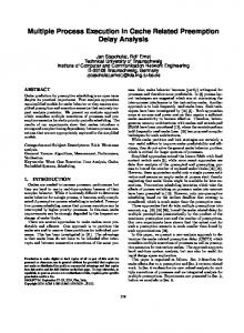
(otherwise it will have to wait further). When τ j starts its execution, it does not preempt τi either directly or nestedly, but inhibits the preempted task τi from resuming its execution. We term this scenario, not yet addressed in the literature, as an inhibiting preemption of task τi by task τ j . A task τ j can inhibitingly preempt only one lower priority task (just like in a direct preemption). Figure 1 shows an example of inhibiting preemption. The upward arrow ↑ denotes the release of a job of a particular task. In this figure, a job of task τ1 directly preempts the job of task τ3 at time ta . This job of task τ1 finishes at time tb and at exactly the same time, a job of task τ2 is released, which inhibits the already preempted job of task τ3 from resuming its execution (Note- The task τ2 could have been released at any time during [ta , tb ] so as to inhibit τ3 at tb ). Here, we can say that the task τ2 inhibitingly preempts task τ3 at time tb . At time tc , the execution of job of task τ2 is over and the preempted job of task τ3 resumes.

Figure 1: Inhibiting preemption

Every invocation of all higher priority tasks during the response time of (a job of) task τi can be categorised into one of the three types of preemptions of τi : direct, nested or inhibiting. The term non-nested preemptions group together the direct and inhibiting preemptions. As nested preemptions are transitive, counting the same invocation of a higher priority task multiple times (as a nested preemption of many lower priority tasks) should be avoided. In earlier works, the number of invocations of higher priority tasks is taken as an upper bound on the number of preemptions of a task which include nested preemptions as well. In this work, we propose that the number of non-nested preemptions (direct + inhibiting) can be taken as a safe and better upper bound on the number of actual (i.e. direct) preemptions. 4. Integration of Non-Nested Preemptions (NNP) and CRPD with Response Time Analysis We first present a method to calculate upper and lower bounds on the number of non-nested preemptions without considering the Cache Related Preemption Delay (CRPD). In section 4.2, a set of constraints based on the bounds on non-nested preemptions are defined. In section 4.3, CRPD is modelled as an optimization problem that maximizes an objective function using the set of constraints. 4.1. Calculation of Non-Nested Preemptions We extend our existing task model by considering an execution time interval [Cimin , Cimax ] for each task τi . Cimin is τi ’s minimum or best case execution time, BCET, and Cimax is maximum or worst case execution time, WCET. The response time equation (1) to calculate the worst case response time (WCRT) can then be re-written as : Ri = Cimax +

 ⎡⎢⎢ Ri ⎤⎥⎥ ⎢⎢⎢ ⎥⎥⎥ × C max j ⎢⎢⎢ T j ⎥⎥⎥ j∈hp(i)

(2)

625

Ravindra B. Keskar et al. / Procedia Computer Science 57 (2015) 622 – 629

We denote the fixed-point (if it exists) for the equation (2) as Rmax . Likewise, to calculate the best (minimum) i response times for a task τi , best case execution times (BCET) Cimin for every task τi and all its higher priority tasks are assumed. Also, as shown by Redell et.al. [9], a favorable instant needs to be considered for the best possible task phasing. A favorable instant occurs for a task τi at its finishing time T if if a job of τi starts execution right upon its release and its completion time coincides with the simultaneous release of all higher priority tasks. The response time analysis equation for the best case response time (BCRT) [9] is given as follows. Ri = Cimin +

 ⎡⎢⎢ Ri − T j ⎤⎥⎥ min ⎥ ⎢⎢⎢ ⎢⎢⎢ T j ⎥⎥⎥⎥⎥ × C j

(3)

j∈hp(i)

To solve equation (3), the fixed-point Rmax calculated by equation (2), is assumed as the first guess for the response i time Ri . This leads to a monotonically non-increasing function and it’s fixed-point provides the tightest (highest) lower bound on the best case response time. This fixed-point is denoted as Rmin i , the best-case response time (BCRT) for task τi . min Let I max j,i and I j,i denote respectively the maximum and minimum number of invocations (releases) of a higher priority task τ j during response time of τi , across all phases. Then, ⎡ max ⎤ ⎢⎢⎢ Ri ⎥⎥⎥ ⎥⎥ I max = ⎢⎢⎢⎢ j,i ⎢ T j ⎥⎥⎥ ⎤ ⎡ ⎤ ⎡ min ⎢⎢⎢ Ri − T j ⎥⎥⎥ ⎢⎢⎢ Rmin i ⎥⎥⎥⎥ ⎥ ⎢ ⎢ I min = −1 = j,i ⎥⎥⎥⎥ ⎢⎢⎢⎢ T j ⎥⎥⎥⎥ ⎢⎢⎢⎢ Tj

(4a) (4b)

Let N j,i denote the number of non-nested (direct + inhibiting) preemptions of a job of task τi by task τ j , in some min execution of τi . Let N max j,i and N j,i respectively denote the upper and lower bounds for N j,i in any execution of τi (i.e. max max across all possible phases). Trivially, 0 ≤ N min j,i ≤ N j,i ≤ N j,i ≤ I j,i ( j < i). min 4.1.1. Calculation for N max j,i and N j,i min The upper and lower bounds on non-nested preemptions, respectively N max j,i and N j,i , can be calculated using equations given below: max max N1,2 = I1,2 = Rmax 2 /T 1 

(5a)

min min N1,2 = I1,2 = (Rmin 2 /T 1  − 1)0 ⎛ ⎞ i−1 ⎜⎜⎜ ⎟⎟  ⎟⎟ min min ⎟ ⎜⎜⎜⎜I max − = (N × I ) N max ⎟⎠ j,i j,k k,i ⎟ ⎝ j,i

(5b)

N min j,i

(5c)

k= j+1

0

k= j+1

0

⎛ ⎞ i−1 ⎜⎜⎜ ⎟⎟⎟  ⎜ min max max = ⎜⎜⎜⎝I j,i − (N j,k × Ik,i )⎟⎟⎟⎟⎠

(5d)

min where (x)0 = max(0, x). The values of N max j,i and N j,i are calculated in the decreasing order of priority for all tasks τi . min In equation (5c), by definition, the term N j,k denotes the minimum or guaranteed number of non-nested preemptions of an intermediate priority task τk ( j < k < i) by τ j during response time Rk of task τk across all phases. The term min min denotes the minimum number of invocations of τk in any response time of τi . Hence the expression (N min Ik,i j,k × Ik,i ) denotes the minimum guaranteed number of non-nested preemptions of τk by τ j during any response time of τi . Summing this term ∀k, ( j < k < i), gives the minimum guaranteed number of non-nested preemptions effected by τ j in all tasks with priority higher than τi (but lower than τ j ) during any response time of τi . We note that, all the non-nested preemptions of tasks τk (∀k, j < k < i) by τ j , are nested preemptions for τi during its response time. Hence, subtracting the above sum (that represents minimum guaranteed number of nested preemptions due to τ j in any response time of τi ) from I max j,i (maximum possible invocations of τ j in any response time of τi ), gives the maximum non-nested preemptions of τi by τ j in the response time of τi . Symmetrically, the equation (5d) can be explained that calculates the minimum guaranteed preemptions of τi by τ j during the response time of τi . It can be proved by induction that min the values of N max j,i and N j,i calculated by equations (5c) and (5d) are respectively the upper and lower bounds on the number of non-nested preemptions of τi by τ j during response time of τi , without considering CRPD cost, across all phases.

626

Ravindra B. Keskar et al. / Procedia Computer Science 57 (2015) 622 – 629

Example 4.1. Consider the taskset given in Table 1. Assume Cimax = Cimin for each task τi . Using equations (2) to Table 1: Task-Set Example Task τi τ1 τ2 τ3

Cmax = Cmin i i 2 8 15

Period T i 7 20 100

(5d), we get : Rmax =2 1 Rmax 2 Rmax 3

= 12 = 55

Rmin 1 = 2 Rmin 2 Rmin 3

max I1,2 = E1 (R2 ) = 2

= 10

max I2,3 max I1,3

= 43

min I1,2 =1

= E2 (R3 ) = 3

min I2,3 min I1,3

= E1 (R3 ) = 8

=2

max N1,2 =2

min N1,2 =1

=3

min N2,3 =2

=6

min N1,3 =1

max N2,3 max N1,3

=6

min is 1, which implies at-least one guaranteed non-nested preemption of τ2 by τ1 during response The value of N1,2 min min min , i.e. 2 non-nested preemptions of τ2 by τ1 are guaranteed in response time of τ3 . = 2, N1,2 × I2,3 time of τ2 . As I2,3 max max max These are nested preemptions for τ3 and as I1,3 = 8, we get N1,3 = 6. Thus, the term N1,3 gives an upper bound on max . the non-nested preemptions of τ3 by τ1 and is lower than the maximum number of invocations of τ1 in τ3 , i.e. I1,3 max Let N j,i represent the actual number of non-nested preemptions of task τi by higher priority task τ j . As N j,i and N min j,i represent respectively upper and lower bounds on N j,i , we have max N min j,i ≤ N j,i ≤ N j,i

(6)

If the total number of preemptions faced by a task τi due to all the higher priority tasks during its response time Ri is represented as Ni . Let Nimax and Nimin represent upper and lower bounds on Ni , then we have: Nimin ≤ Ni ≤ Nimax

(7)

where Ni =

i−1 

N j,i

and

Nimax =

j=1

i−1 

N max j,i

and

j=1

Nimin =

i−1 

N min j,i

(8)

j=1

Let the actual number of non-nested preemptions of task τi by task τ j during response time Rk of a lower priority max task τk ( j < i < k), be denoted by k N j,i and bounded by k N min j,i and k N j,i as follows: min k N j,i

where

≤ k N j,i ≤ k N max j,i

⎡ max ⎤ ⎢⎢⎢ Rk ⎥⎥⎥ max ⎥⎥ × N max N = ⎢⎢⎢⎢ k j,i j,i ⎢ T i ⎥⎥⎥

and

⎞ ⎛⎡ min ⎤ ⎟ ⎜⎜⎜⎢⎢ Rk ⎥⎥ min ⎥⎥⎥ − 1⎟⎟⎟⎟ × N min ⎢⎢ ⎜ N = ⎜ ⎢ k j,i ⎠ ⎝⎢⎢ T ⎥⎥ j,i ⎢ i ⎥

(9)

(10)

The total number of preemptions faced by a task τi due to its higher priority tasks during the response time Rk of a lower priority task τk is represented as k Ni and is bounded by k Nimax and k Nimin as: min k Ni

≤ k Ni ≤ k Nimax

The terms k Nimax and k Nimin can be calculated as: max k Ni

⎡ ⎤ ⎢⎢ Rk ⎥⎥ = ⎢⎢⎢⎢ ⎥⎥⎥⎥ × Nimax ⎢⎢ T i ⎥⎥

and

min k Ni

(11)

⎛⎡ ⎤ ⎞ ⎜⎜⎢⎢ Rk ⎥⎥ ⎟⎟ = ⎜⎜⎝⎢⎢⎢⎢ ⎥⎥⎥⎥ − 1⎟⎟⎠ × Nimin ⎢⎢ T i ⎥⎥

Given below are a set of constraints based on the terms defined here.

(12)

627

Ravindra B. Keskar et al. / Procedia Computer Science 57 (2015) 622 – 629

4.2. Set of Constraints As the number of non-nested preemptions of every task τi by all of its higher priority tasks τ j during response time Rk of a lower priority task τk , is less than or equal to the number of invocations of all the higher priority tasks τ j during Rk , we have the following inequality: ⎡ ⎤ ⎢⎢⎢ Rk ⎥⎥⎥ ⎢⎢⎢ ⎥⎥⎥ N ≤ k j,i ⎢⎢ T j ⎥⎥

(13)

i = 2, 3, . . . , k j = 1, 2, . . . i − 1

The number of non-nested preemptions of τi by τ j in Rk (i.e. k N j,i ) is less than or equal to the number of invocations of τ j during Ri multiplied by the number of invocations of τi during Rk . Hence, we have: k N j,i

⎡ ⎤ ⎡ ⎤ ⎢⎢ Ri ⎥⎥ ⎢⎢ Rk ⎥⎥ ≤ ⎢⎢⎢⎢ ⎥⎥⎥⎥ × ⎢⎢⎢⎢ ⎥⎥⎥⎥ ⎢⎢ T j ⎥⎥ ⎢⎢ T i ⎥⎥

(14)

i = 2, 3, . . . , k j = 1, 2, . . . i − 1

Combining equations (9), (13) and (14), we have min k N j,i

⎛⎡ ⎤ ⎜⎜⎢⎢ Rk ⎥⎥ ≤ k N j,i ≤ min ⎜⎜⎝⎢⎢⎢⎢ ⎥⎥⎥⎥, ⎢⎢ T j ⎥⎥

⎡ ⎤ ⎡ ⎤ ⎞ ⎢⎢⎢ Ri ⎥⎥⎥ ⎢⎢⎢ Rk ⎥⎥⎥ ⎟⎟⎟ ⎢⎢⎢ ⎥⎥⎥ × ⎢⎢⎢ ⎥⎥⎥, k N max ⎟⎠ j,i ⎢⎢ T j ⎥⎥ ⎢⎢ T i ⎥⎥

(15)

i = 2, 3, . . . , k j = 1, 2, . . . i − 1 max To calculate the values of k N min j,i and k N j,i , equations (5c), (5d) and (10) can be used. The total number of preemptions of tasks τ2 , τ3 , . . . , τi during response time Rk of task τk cannot be greater than the number of invocations of higher priority tasks τ1 , τ2 , . . . , τi−1 during Rk . l 

k Ni

≤

i=2

⎤ l−1 ⎡  ⎢⎢⎢ Rk ⎥⎥⎥ ⎢⎢⎢ ⎥⎥⎥ ⎢⎢ T j ⎥⎥

(16)

j=1

l = 2, 3, . . . , k

The number of preemptions caused by task τ j during response time Rk of task τk is less than or equal to the number of invocations of τ j during Rk . k 

k N j,i

i= j+1

⎡ ⎤ ⎢⎢ Rk ⎥⎥ ≤ ⎢⎢⎢⎢ ⎥⎥⎥⎥ ⎢⎢ T j ⎥⎥

(17)

j = 1, 2, . . . , k − 1

4.3. Calculation of CRPD and Response Time The CRPD cost of a single preemption of task τi due to higher priority task τ j , denoted by f j,i , can be given by using ECB-Union method [7].

⎛ ⎞



⎜ ⎟⎟⎟

⎜⎜  f j,i =

⎜⎜⎜⎜⎝ ECBh ⎟⎟⎟⎟⎠ ∩ UCBi



h∈hp( j)∪{ j}

(18)

The total number of cache blocks replaced during response time Rk of task τk can be calculated by maximizing the objective function: PCk (Rk ) =

i−1  k  

k N j,i

× f j,i



(19)

i=2 j=1

Here, PCk (Rk ) denotes a guaranteed upper bound on the number of cache blocks replaced during response time Rk of task τk . This includes the number of cache blocks replaced due to preemptions of τk and higher priority tasks τ2 , . . . τk−1 . The values of the terms k N j,i can be calculated by solving the constrains (inequalities) given by equations (13) to (17) and maximizing the objective function given by equation (19). This can be done by using integer linear programming method and tools like LPSolve [10]. The response time for task τk that includes its CRPD cost can be calculated iteratively as a fixed-point solution to the equation below where the worst case execution time of τk , i.e. Ck , is considered as the initial value of Rk . Rk = C k +

 ⎡⎢⎢ Rk ⎤⎥⎥ ⎢⎢⎢ ⎥⎥⎥ × C j + (PC (R ) × BRT ) k k ⎢⎢⎢ T j ⎥⎥⎥ j∈hp(i)

6

(20)

628

Ravindra B. Keskar et al. / Procedia Computer Science 57 (2015) 622 – 629

Here, BRT stands for Block Reload Time, an upper bound on the time required to reload a single cache block. The response time equation (20) is solved by considering tasks in the decreasing order of priority. As calculation of N max j,i max and N min and Rmin respectively, we j,i terms require availability of both maximum and minimum response times Ri i propose the following algorithm that integrates CRPD costs into the worst response time analysis. min Algorithm 1 Rmax with CRPD using Integer Linear Programming and values of N max i j,i / N j,i

1: Rmax ← C1max ; 1 min 2: Rmin 1 ← C1 ; 3: for i = 2 to N do 4: Calculate fixed-point for Rmax (without CRPD) using equation (2); i 5: Calculate fixed-point for Rmin (without CRPD) using equation (3); i max 6: Ri ← Ci ; 7: while (fixed-point for Ri is not reached and Ri < Di ) do 8: for j = 1 to i-1 do 9: Calculate N max j,i using equation (5c) and current Ri ; 10: Calculate N min j,i using equation (5d); 11: Calculate CRPD value PCi (Ri ) by maximizing the objective function given by equation (19); 12: //Use equation (18) and solve constraints in equations (13) to (17); 13: end for 14: Calculate new Ri with Equation (20), using PCi (Ri ) value calculated in step 11 and current Ri ; 15: end while 16: if Ri > Di then 17: break; 18: end if 19: end for

5. Comparison with methods by Lee et.al. The technique by Lee et.al. [4] categorizes the preemptions of a task into a number of disjoint groups, where each of these groups correspond to a preemption scenario. They have introduced a term gRj i (H) that denotes the number of preemptions of τ j when task set H executes during Ri . A set of constraints are defined on gRj i (H) terms which are solved using ILP techniques. As the number of scenarios are exponential with respect to the number of higher priority tasks, the number of gRj i (H) terms are also exponential. The set of constraints defined as such may sometimes lead to infeasible and pessimistic solutions. This is due to lack of a constraint to limit the number of times a particular higher priority task τ j is involved in preemptions of lower priority tasks (number of disjoint scenarios H) during Ri . Direct addition of such a constraint to the system leads to double counting of some terms and hence to an unsafe solution. The double counting is removed by an independent and exponential analysis. Finally, Lee et.al. [4] suggested a technique to independently consider phasing effects of different tasks with respect to each other. In summary, it can be said that the method given by Lee et.al. [4] is a technique that involves analysis of an exponential number of terms. Hence its complexity is exponential with respect to the number of tasks in the taskset (O(2N )). The differences between our method and method by Lee et.al. [4] are as follows: 1. The number of terms involved and the overall analysis by Lee et.al. is exponential with respect to the number of tasks in a taskset. On the other hand, the number of k N j,i terms (∀ j < i, i < k, k < N) used in the objective function proposed by us in equation (19) are polynomial (O(N 3 )) with respect to the number of tasks in the taskset. The overall complexity of our method is pseudo-polynomial due to the use of Response Time Analysis (RTA) framework and Integer Linear Programming. 2. In our method, the number of non-nested preemptions are bounded from above as well as below, respectively min by k N max j,i and k N j,i . The constraint given by us in equation (17) naturally restricts the number non-nested preemptions due to task τ j to be lower than or equal to the number of invocations of task τ j . This avoids infeasible solutions and also avoids independent removal of double counting of terms with exponential analysis required by the method of Lee et.al. min 3. By definition, as N max j,i and N j,i terms are the upper and lower bounds on non-nested preemptions across all possible phases, phasing effects need not be considered separately as is done in the method of Lee et.al [4].

Ravindra B. Keskar et al. / Procedia Computer Science 57 (2015) 622 – 629

5.1. Experimental Set-up We randomly generated 1000 synthetic task sets such that utilization of tasks within a task set are uniformly distributed using UUnifast algorithm[11]. The default taskset size is assumed to be 10. Task periods are generated according to a log-uniform distribution with a minimum period of 20ms and maximum period of 500ms, which are typical for automotive applications. Task deadlines are implicit, i.e. Di = T i and the priorities are assigned in the deadline/rate monotonic order. The worst task execution times are based on the utilization and period selected: Cimax = Ui × T i . We also assume Cimax = Cimin , i.e. WCET = BCET. We assume that the number of cache-blocks or cache-sets (CS) is 256 and the Block Reload Time (BRT) is 8 μs. Total cache utilization CU = 10, implying that the total memory blocks required by all the tasks together is (CS × CU). The ECBs are generated using the UUnifast [11] algorithm. The ECBs of each task τi are assumed to be consecutively arranged starting from a random cache block S to (S + |ECBi |) modulo CS. The reuse factor RF gives a measure for reuse of cache blocks. The UCBs for every task τi are generated according to a uniform distribution in the range [0, RF × |ECBi |] with RF=0.3. An initial set of results and trends can be summarized as follows. Our proposed method can schedule some tasksets that the method by Lee et.al. (without using exponential analysis for removal of double counting) cannot and also vice versa. The method by Lee et.al. that removes infeasible solution, double counting of terms and phasing effects using independent exponential analyses performs better than our method. This is because, as the exponential number of terms and all possible scenarios are considered by Lee et.al., the cost of preemption calculated for each scenario is more fine-grained. On the other hand, our method has a polynomial number of terms and hence the run-time of our method is found to be almost 15-20 times lower than both variants of methods by Lee et.al., with or without the removal of infeasible solutions and double counting. These results imply that our method naturally gives more feasible results with better efficiency: requiring much lower run-time and avoiding separate calculations for double counting or phasing effects. These trends also imply that there is a scope for improvement in our method by considering more exhaustive scenarios and fine-grained CRPD cost for each scenario which may lead to more accurate results. More experimentation is required to be done to identify scenarios where each method becomes incomparable with respect to the other, that is, when a method can schedule tasksets not schedulable by other methods. 6. Conclusion In this paper, we presented a novel technique to calculate non-nested preemptions that provides upper and lower bounds on the number of preemptions of a task. We then used these bounds to define a set of constraints that can be solved using ILP techniques to calculate the CRPD values. We also presented an algorithm to integrate these CRPD values into the worst response time analysis. Future work involves making our analysis more accurate and comparing our method with multiset-based analytical techniques in [7]. References [1] J.V.Busquets-Mataix, J.J.Serrano, R. Ors, P. Gil, A. Wellings, Adding instruction cache effect to schedulability analysis of preemptive realtime systems, in: Proceedings RTAS, 1996, pp. 204–212. [2] Y. Tan, V. Mooney, Timing analysis for preemptive multi-tasking real-time systems with caches, ACM Trans. Embedded Comput. Syst. 6(1):1210275. [3] C. Lee, J. Hahn, Y. Seo, S. Min, R. Ha, S. Hong, Y. Park, M. Lee, C. S. Kim, Analysis of cache-related preemption delay in fixed-priority preemptive scheduling, IEEE Transactions on Computers 47(6) (1998) 700–713. [4] C. Lee, J. Hahn, Y. Seo, S. Min, R. Ha, S. Hong, Y. Park, M. Lee, C. S. Kim, Bounding cache-related preemption delay for real-time systems, IEEE Trans Software Engg 27(9) (2001) 805–826. [5] H. Ramaprasad, F. Mueller, Tightening the bounds on feasible preemptions, ACM Trans. Embedded Comput. Syst. 10(2) (2010) 27:1–30. [6] J. Staschulat, S. Schliecker, R. Ernst, Scheduling analysis of real-time systems with precise modeling of cache related preemption delay, in: Euromicro Conference on Real-Time Systems (ECRTS’05), 2005, pp. 41–48. [7] S. Altmeyer, R. Davis, C. Maiza, Improved cache related preemption delay aware response time analysis for fixed priority pre-emptive systems, Real Time Systems 48 (June 2012) 499–526. [8] M. Joseph, P. Pandya, Finding response times in a real-time system, Comput J 29(5) (1986) 390–395. [9] O. Redell, M. Sanfridson, Exact best-case response time analysis of fixed priority scheduled tasks, in: ECRTS ’02: Proceedings of the 14th Euromicro Conference on Real-Time Systems, 2002, pp. 165–172. [10] Lpsolve, http://sourceforge.net/projects/lpsolve/. [11] E. Bini, G. Buttazzo, Measuring the performance of schedulability tests, Real Time Systems 30 (2005) 129–154.

629