[11] William Henderson, David Kendall, and Adrian Robson. Improving the accuracy of scheduling analysis applied to distributed systems computing minimal ...
Multiple Process Execution in Cache Related Preemption Delay Analysis Jan Staschulat, Rolf Ernst Technical University of Braunschweig Institute of Computer and Communication Network Engineering D-38106 Braunschweig, Germany {staschulat,ernst}@ida.ing.tu-bs.de ABSTRACT
cess. Also, cache behavior becomes (partly) orthogonal for processes and therefore more predictable. In [6] process layout techniques are suggested which aim at minimizing the inter-process interference in the instruction cache. Another approach is to lock frequently used cache lines. Such techniques have been investigated by [14] [5] . Both approaches come at an area and power cost as they require a sufficient cache associativity to become effective. Therefore, heterogeneous memory architectures with caches and scratch-pad SRAM have been introduced [12], where the scratch-pad can hold frequently used cache lines. [19] has proposed compiler techniques for such architectures. While cache partition and lock strategies are certainly a very useful add-on to improve cache predictability and efficiency, they do not solve the general cache behavior problem which is critical for larger systems of processes. Simplified approaches extend the known RMA with fixed context switch costs [3], while more recent approaches use data flow analysis of the preempted and preempting process to bound the number of replaced cache blocks [16] [18]. However, these approaches model only a single process activation and assume an empty cache at process start thereby neglecting that cache blocks might be available for later executions. Pre-runtime scheduling heuristics which take the effects of process switching on processor cache into account have been presented in [13]. However, only non-preemptive scheduling based on the earliest deadline first strategy is considered, which is much easier than the preemptive case. Those approaches that do take multiple preemptions into account, e.g. [18] [16] [26], bound the cache related delay for multiple preemptions pessimistically by the product of the maximum preemption cost and the number of preemptions. Our own experiments have shown that the actual cost for such a preemption scenario is much smaller than found by such approximations [24]. In this paper, we present a new analysis approach to determine the cache related preemption delay (CRPD) which considers multiple executions of processes as well as preemption scenarios for instruction caches. The approach supports hard real-time system analysis, but can also be useful for rapid design space exploration. This paper is organized as follows. Sec. 2 describes the cache effects due to a preemption and Sec. 3 reviews related work. In Sec. 4 we describe our new refined analysis for multiple executions of processes and an integrated analysis for multiple preemptions. Experiments are presented in Sec. 5, before we conclude in Sec. 6.
Cache prediction for preemptive scheduling is an open issue despite its practical importance. First analysis approaches use simplified models for cache behavior or they assume simplified preemption and execution scenarios that seriously impact analysis precision. We present an analysis approach which considers multiple executions of processes and preemption scenarios for static priority periodic scheduling. The results of our experiments show that caches introduce a strong and complex timing dependency between process executions that are not appropriately captured in the simplified models. Categories and Subject Descriptors: B.3.3: Worst-case analysis. General Terms: Algorithms, Measurement, Performance, Verification. Keywords: Worst Case Execution Time Analysis, Cache, Embedded Systems, Scheduling.
1.
INTRODUCTION
Caches are needed to increase processor performance but they are hard to use in real-time systems because of their complex behavior. While it is already difficult to determine cache behavior for a single process, it becomes really complicated if preemptive process scheduling is included. Preemptive process scheduling means that process execution can be interrupted by higher priority processes. In this case, cache improvements can be strongly degraded by the frequent exchange of cache blocks. There are several approaches to make caches more predictable and efficient. One approach is to partition the cache sets and to reserve these partitions for individual processes. This has been investigated in [21]. The advantage is that cache lines do not have to be reloaded after interrupts and between consecutive executions of the same pro-
Permission to make digital or hard copies of all or part of this work for personal or classroom use is granted without fee provided that copies are not made or distributed for profit or commercial advantage and that copies bear this notice and the full citation on the first page. To copy otherwise, to republish, to post on servers or to redistribute to lists, requires prior specific permission and/or a fee. EMSOFT’04, September 27–29, 2004, Pisa, Italy. Copyright 2004 ACM 1-58113-860-1/04/0009 ...$5.00.
278
2.
PROBLEM DESCRIPTION
higher priority processes are considered in CRPD- and scheduling analysis. But this simplification is only acceptable if an empty cache is assumed at every process start. It is not acceptable for processes with linear code which are activated multiple times: the worst case response time will be overestimated and unsuitable for the design and verification of realistic embedded systems. Therefore we developed a new approach, which considers the cache state at process start. Consider Fig. 1. After the first activation of P2 , some cache blocks can be replaced by the lower priority process P3 and available cache blocks for the second activation of P2 reduce the number of compulsory cache misses. Preemptive scheduling analysis has to consider the WCET, direct context switch costs of the operation system and the indirect cache related preemption delay. The CRPD depends on the frequency and location of preemptions as well as the additional time delay for reloading replaced cache blocks.
This work considers a single processor system with preemptive scheduling. In Figure 1 a process P2 is activated and finishes execution without preemption. Then a lower priority process P3 executes and P2 is activated again. Another process P1 , which has a higher priority than P2 preempts P2 . P1 finishes execution, and P2 resumes.
P1 P2 P3 useful CB of P2
0
1
2
3 4 5
Time used CB of P1
CRPD
6
7
8
9 0
a b
c
2.2
d
e
Figure 1: Scheduling of three tasks P1 , P2 and P3 . The upper portion displays teh preemption of task P2 by P1 and the lower portion shows the cache contents. This preemption can take place anytime during execution of P2 . In rate monotonic scheduling shorter processes have a higher priority which lead to multiple preemptions of a lower priority process, such as P2 . In the lower part of Fig. 1, a direct mapped cache with 16 cache blocks is shown. The cache behavior during the preemption is described in Sec. 2.3. In this paper we only analyze instruction caches.
2.1
Preemption frequency and location
The number of preemptions depends essentially on the scheduling strategy and the operating system. In this paper we consider only static priority periodic scheduling and assume the number of preemptions to be known a priori. This is not a limitation, since the approach can be coupled with an iterative response time analysis, as proposed for a wide range of scheduling strategies, for example [4]. Preemptions can take place anytime. Therefore a lower priority process can be preempted anywhere except where preemptions are explicitly disabled, such as in protected program segments. The space of possible preemption points is Time flow graph (CFG) of the process, where given by the control nodes represent basic blocks of the process and edges the control flow dependency. In this work we assume at most one preemption at each basic block, as in [15]. We argue in Sec. 4.1 why this is correct, even though several preemptions might take place in long basic blocks.
2.3
Preemption cost
The time delay for one preemption depends on the preempted process P2 , the preempting process P1 , and the instruction cache state at the start of process P2 . Only useful cache blocks can lead to additional cache misses, where a useful cache block at an execution point is defined as a cache block that contains a memory block that may be rereferenced before being replaced by another memory block [16]. For example, it is possible that the replaced memory block is one that is no longer needed or one that will be replaced without being re-referenced, even when there were no preemptions. The number of useful cache blocks depends on the control flow structure. All cache blocks that hold memory blocks of a loop body are useful, provided that the entire loop body fits in the cache. The number of useful cache blocks within a basic block of a sequential process is at most one at every execution point if an empty cache is assumed at process start. Additionally, one cache miss occurs if a preemption replaces the cache block, which contains the instructions of the current basic block. The second influence is induced by the preempting process. Only the cached memory blocks of process P1 replace cache blocks of process P2 . The execution path of P1 that uses the maximum number of cache blocks has been considered as the worst case for the preempting process [26].
Application domain
Current analysis techniques, which are reviewed in Sec. 3, model each process in isolation and assume pessimistically an empty cache at process start. The WCET of the process is overestimated, because compulsory cache misses might not be necessary for the next activation. This might possibly be acceptable for processes with computation intensive loops such as those found in large filter algorithms, MPEG decoding or sorting algorithms. However, typical automotive real time applications, such as engine control, consist of linear code without loops that are activated periodically by the operating system. This property is not limited to automotive applications, as those generated from Matlab/Simulink, Petri-nets or ASCET/SD often posses this property. This linearity leads to a fundamentally different cache behavior. A cache does not speed up linear code, since memory lines are executed sequentially and only once. The speedup is gained only if the cache holds memory lines from an earlier process activation. In the best case, all memory lines are present in the cache and a second activation requires no further instruction cache misses. The second drawback of current approaches is that only
279
The worst case CRPD for one preemption is given by the intersection of the maximum number of useful cache blocks of process P2 and the used cache blocks of process P1 multiplied by the constant cache refill time at a given preemption point p1 . In our example the preemption cost CRP DPP21 (p1 ) where process P1 preempts P2 at preemption point p1 is defined by CRP DPP21 (p1 ) = tref ill · |U CBP2 (p1 ) ∩ U BP1 |
each preemption separately. Thus, the important case of multiple process executions is not considered. Another approach [26] concentrates on the analysis of used cache blocks of preempting process P1 using an ILP technique and classifies all cache blocks of the preempted process P2 as useful. Multiple preemptions are not considered and a cold cache is assumed at process start. [18] refines the data flow analysis of [16] and extend the approach of [26] by modeling the cache content as a state instead of a set. All possible cache states of the preempting and preempted process are intersected to find the maximum CRPD. Multiple preemptions are not considered and an empty cache is assumed at process start. [22] uses the same worst case assumption based on cache analysis by [9] but uses a more precise context switch model, including deep pipeline scheduling. A simulation based method is suggested in [7], which uses live cache frames to bound the number of replaced cache blocks. Again, an empty cache at process start and a single delay for all preemptions is considered. Currently the preempting and preempted process are accurately analyzed by data flow analysis enhanced by considering several paths in the control flow graph. However, above approaches assume an empty cache at process start. This is very pessimistic, since processes in real time embedded systems are activated multiple times. Existing cache blocks from earlier executions can reduce the number of cache misses in later executions substantially. Current approaches either model only the number and cost of preemptions or multiple process execution without preemption delay, but no approach models both situations. Only the combination of both effects provides sufficient accuracy, as we will see in the experimental results.
(1)
where tref ill denotes the cache refill time, U CBP2 (p1 ) the set of useful cache blocks of process P2 at p1 and U BP1 the set of used cache blocks of process P1 . Fig. 1 presents the cache contents for P1 and P2 . Cache blocks 0 -9 are useful cache blocks (CB) of P2 at the preemption point and CB 5 - c are the used cache blocks of P1 . The intersection (CB 5-9) are the cache blocks that are reloaded when P2 resumes execution. In this case the CRPD is five cache misses. Then, for a given number n of preemptions, the total CRPD assumed by [16] [18] [26] is given by n · maxpi CRP DPP21 (pi )
(2)
The drawback of such a pessimistic model is using the maximum time delay for every preemption. This greatly overestimates the actual preemption cost. We have seen in experiments that the preemption cost tends to drop significantly for multiple preemptions [24]. Consider two preemption points p1 and p2 with the same number of useful cache blocks (not shown in the figures). If a preemption at p1 replaces them all then a preemption at p2 cannot replace even one, because all useful cache blocks have already been replaced. So the preemption cost at p2 is zero. In general, the preemption cost of the nth preemption depends on the replaced cache blocks of all n−1 previous preemptions. This will be further analyzed in Sec. 4.3. Before we present our approach in Sec. 4 we review related work.
3.
4.
REFINED APPROACH
The refined approach addresses two aspects in cache related preemption delay analysis: (1) the cost of preemption scenarios and (2) the cache state at process start, to consider multiple process activations. A preemption scenario (P2 , P1 , {p1 , · · · , pn }) is a 3-tuple of the preempted process P2 , the preempting process P1 and the set of preemption points {p1 , · · · pn }. A preemption point pi is a basic block in the CFG of the process P1 , like in [16]. The assumptions of our approach are summarized in Sec. 4.1. The analysis of a single preemption is described in Sec. 4.2 for direct mapped and m-way set associative caches. Sec. 4.3 describes our approach for preemption scenarios and Sec. 4.4 for multiple process activations. Finally the computation of the worst case preemption scenario is presented in Sec. 4.5.
RELATED WORK
Early work on cache behavior for a single process does not take preemption into account [17] [9] [28] [27]. First proposals for cache modeling and timing analysis use simplified cache models. [2], [3] and [20] extend the known RMA by a fixed context switch cost. [15] uses data flow analysis to determine the CRPD when a process P1 preempts process P2 by analyzing the number of useful cache blocks of P2 . Then, a complex analysis follows, analyzing all possible combinations of preemptions. The cost of multiple preemptions is determined by the sum of the n most expensive preemptions assuming all useful cache blocks to be replaced. They refine their approach in [16], by intersecting the number of useful cache blocks of P2 with the number of used cache blocks of P1 . However, to cope with the computational effort of their complex preemption model the computation of multiple preemptions is simplified to multiplying the maximum preemption cost by the number of preemptions. The number of preemptions is determined by integer linear programming (ILP) and process phasing based on worst case and best case response time (BCRT) of processes. However, the BCRT analysis is a complicated problem where only approximative solutions have been proposed for the general case ([11] [10]) and the BCRT determination is not described by the authors. Unfortunately, they don’t publish experiments showing the accuracy of this model. Furthermore, both versions assume an empty cache at process start and analyze
4.1
Assumptions
Our approach has five main assumptions: 1. The worst case scenario does not contain two preemptions in the same execution of a basic block. This simplification can be justified by the following consideration. Suppose thee are m preemptions during the execution of a large basic block bi . The total preemption cost is then bounded by C = maxCRP D(bi ) + m
(3)
cache misses. That is, the maximum cache related preemption delay of bi plus m cache misses for the m
280
preemptions of the block that possibly require reload of the current cache block when that basic block is continued. The reason is that a basic block consists only of sequential code and at most one cache block is useful at any time during its execution. Therefore, the maximum CRPD for each additional basic block preemption is equal to or less then any other preemption in the process. As long as there are still basic blocks that have not been preempted, this assumption does not change the maximum preemption cost. This assumes that there are more basic blocks than preemptions by another process, which we consider to be true for real-life control flow graphs. It is obviously easy to detect situations in which this assumption does not hold and equally easy to add the corresponding 1 cache miss per additional preemption. So, this assumption is not a limitation.
Similarly LCS is computed by an iterative fixed point algorithm. RCSB captures the possible cache states when P is preempted and LCSB captures the possible cache usages when P resumes execution. The intersection of both sets is the set of useful cache blocks of basic block B. The used cache blocks of a preempting process P 0 is given by RCSend , assuming end is the last basic block of P 0 . Finally the CRPD at a basic block B is computed by the intersection of used cache blocks and useful cache blocks.
Control flow graph
U: -
RCSend(P1): cb 5-8, b-c
cb 7-8
U: 8
cb 5-6, 9-c
cb 8-9
Figure 2: Analysis of useful and used cache blocks
Fig. 2 shows a small control flow graph of process P1 and P2 , where memory lines for basic block 3 map to cache lines 7 - 8 and memory lines from basic block 4 map to cache lines 8 - b. Therefore at b3 cache line 8 is useful. We assume that cache line 8 is also useful at b4 . On the right side the used cache blocks of process P1 are shown. In this case two RCSend states are possible at the last control flow node of P1 . Because cache line 8 is used and useful at node b3 one cache miss would occur, if a preemption takes place at node b3 .
This subsection describes the approach of [18] for direct mapped caches. A cache state denotes the contents of all cache blocks. For a direct mapped cache with n blocks, a cache state is a vector of n elements, where c[i] = m if cache block i contains memory block m. A reaching cache state RCSB at a basic block B of a process is the set of possible cache states when B is reached via any incoming program path. The live cache states at a basic block B, denoted LCSB , are the possible first memory references to cache blocks via any outgoing program path from B. A least fixed point algorithm computes the values of these sets. IN OU T To compute RCS, the quantities RCSB and RCSB are OU T computed and we set RCSB = RCSB if the fixed point is IN OU T reached. Initially RCSB = ∅ and RCSB = genB , where genB holds all memory blocks introduced into the cache by basic block B. The iterative equations are as follows: [ IN RCSB = RCSpOU T (4)
4.2.2
Extention for n-way associative caches
A n-way set associative caches contains sets with n cache blocks each. The RCS and LCS are defined for each cache set. The usefulness of a cache block is determined by comparing the contents of both RCS and LCS. Unlike a directmapped cache, in a n-way set associative cache a memory line can be placed in n different positions in a set. Hence only the cache blocks within a cache set are compared. For example, the content of the first (second, third, ...) block in set 1 in RCS is compared with the contents of all n blocks in set 1 in LCS and so on.
4.3
Multiple preemption cost
We extend the path based CRPD analysis of [18] for preemption scenarios. Suppose that S = {P2 , P1 , {b3 , b4 }} denotes the preemption scenario at basic block b2 and b4 where P1 preempts P2 . At process start we assume an empty cache for now. Fig. 3 shows this preemption scenario. The cost of the first preemption is calculated by the least fixed point algorithm as described in Sec. 4.2. For all further preemptions we procede as follows: To capture the effect of
p∈predecessor(B)
=
cb 1-3
CRPD 1
Direct mapped caches
m m0
bb3
bb4
cb 3-6
U: 8
Single preemption cost
IN {r genB |r ∈ RCSB } 0 0 m if m 6=⊥ m otherwise
bb2
Cache states
To calculate the CRPD for a process, we intersect the set of useful cache blocks of the preempted process with the set of used cache blocks of the preempting process by extending the cache state approach of [18].
=
bb3
U: 3
4. The system uses an m-way associative instruction cache with a deterministic refill strategy (LRU, FIFO) but not a random strategy. In this paper we only analyze the instruction cache. 5. A constant delay time tref ill is assumed for a cache miss.
OU T RCSB
bb1
bb4
3. All processes of the system run between two process activations. This is the worst case for multiple process activations. Future research is necessary for a more precise bound.
4.2.1
P1 (preempting)
bb1 bb2
2. The number of preemptions is given a priori, but this number can formally be bounded by the response time analysis for scheduling algorithms other then fixed priority periodic scheduling, e.g. [4] [3].
4.2
P2 (preempted)
(5) (6)
281
CFG of P2
P1
…
P2 Time useful CB of P2
…
cb 7-8
U: 8
used CB of P1
cb 5-8, b-c
cb 5-6, 9-c
CRPD: 1 0
1
2
3 4 5
6
7
8
9 0
a b
c
d
cache states RCSend of P1
e
Figure 3: Second preemption of process P2 by P1
U: -
cb 8-9 no more useful cache blocks!
a preemption at basic block bi by Pj on later preemptions, a data flow analysis is performed for the preempting process. The cache states of basic block bi are inserted at the first CFG node of Pj . Then the data flow analysis determines all reaching cache states of Pj . The cache states of the last CFG node of the preempting process Pj , RCSend , is the set of used cache blocks of Pj . For each cache state CSk of RCSend , we insert after bi a new basic block node in the CFG of the preempted process and also insert the cache state CSk . If the preempting process Pj finishes with n different reaching cache states then n nodes are inserted. For the inserted node Nk , we define genNk = RCSk , where RCSk is the kth reaching cache state of the last basic block of Pj . For our example in Fig. 1, we see in Fig 3 that only the cache block (CB) of P2 is useful and CB 5 - c are used by P1 . Figure 4 shows a preemption at basic block b3 which uses CB 7 and 8. The preempting process has two cache states at its last node, hence two nodes are inserted. The resulting CRPD is one, because only CB 8 is useful. Then the iterative data flow analysis is applied and the RCS of all other nodes are calculated again. This models the fact that useful cache blocks might be overwritten by a preemption and thus cannot be replaced again. However, the LCS property is not recalculated, because otherwise it would be possible to consider the preempting process’ cache blocks as useful cache blocks. After recalculating the RCSs, the CRPD is calculated for the next preemption point of the preemption scenario. This procedure is applied for every preemption point of the preemption scenario. For loops this analysis is very complex, because several iterations have to be modeled. We can simplify the analysis by considering the number of iterations L and the total number of preemptions n . For the empty cache at process start, the maximum preemption cost will occur within a loop. If L ≥ n then we can precicely calculate the maximum cost by n·CRP Dloop , because all replaced cache blocks are reloaded in the next iteration. CRP Dloop denotes the maximum preemption cost within the loop body. If L ≤ n we can at least conservatively approximate it with n · CRP Dloop . A more accurate analysis would have to unroll the loop L times and consider all possible preemption scenarios, thus increasing the number of possible combinations.
Figure 4: Insertion of nodes in CFG of process P1
4.4
Multiple process execution
In the previous sections we assumed an empty cache at process start. However, some cache blocks might be present in cache when the process is activated a second time. This effects the core execution time of the process itself as well as the CRPD. At first we assume that no processes run between two activations of process Pi . We model a cache state like in Sec. 4.2 by inserting new nodes, but now we insert before the first node in the control flow graph k nodes for k different OU T RCSend values of process Pi .
CFG of P2 … …
Cache states:
bb1
CFG of P3 … …
CFG of P2 … …
bb4
bb1
bb6
bb1
cs i
cs i
cs k
cs k
cs j
cs j
cs l
cs l
cs m
cs m
bb4
Figure 5: Multiple process activation
It is important to consider the processes which run between two activations. In this paper we assume the conservative approximation that all higher priority and lower priority processes of the system can execute. This is new to CRPD analysis, as current techniques consider only higher priority processes. We model the cache behavior of these intermediate execution of Pi , Pj1 , · · · , Pjk , Pi as a sequence of process execuOU T tions. The sets of RCSend of the preceding process Pjm are inserted as start nodes of process Pjm+1 . The last process is the next instance of Pi . Note, that the CRPD at the second activation of process Pj is independent of the order and the
282
˜ 1 , · · · , ni ) E.g., the total cost of all i previous preemptions C(n plus the preemption cost for node ni+1 assuming preemptions at the nodes n1 , · · · , ni . The quality of this algorithm depends on the branchand bound conditions. Branching is controlled by the single preemption cost C(ni ). For a new candidate a node is chosen, which is not taken, e.g., not on this path on the higher levels of the search tree, and has maximum cost, e.g. {nk |C(nk )maximum, nk ∈ L}. The initial bound B of the CRPD for n preemptions is given by iterating equation 7 exactly n times and choosing the most expensive node that is not yet taken. A sub-tree is bounded if the estimated cost after n + 1 i+1 preemption points, Ctotal of eq. 8, is smaller than the current bound B. This means no preemption node is inserted and the search continues at the i − 1th level.
frequency of intermediate processes. (See [25]). Fig. 5 shows two activations of P2 and one intermediate lower priority process P3 corresponding to Fig. 1. The two cache states csi , csj at the end of process P2 are propagated to the first node of the P3 s CFG node. Then the usual data flow analysis determines the RCS states for all nodes. The cache states at the last node csk , csl , csm are again propagated to the beginning of P2 .
4.5
Worst case preemption scenario
This section describes how we find the preemption scenario with the maximum cache related preemption delay. We assume that the preempted process P2 , the preempting process P1 and the number of preemptions n by P1 during execution of P2 is given. The analysis is based on the control flow graph which is constructed by SymTA/P for every process. SymTA/P is a tool to determine the WCET of processes by analyzing feasible pathes on the source code level and is currently being developed at our institute. The architecture can be modeled by an off-the-shelf cycle accurate processor simulator or by measurments on an evaluation board. Further on, a cache analysis determines the worst case cache behavior for m-way associative instruction caches. The longest execution path is found by solving a linear optimization problem based on the control flow graph of the process. For details refer to [27]. Because the total preemption cost for n preemption nodes is not additive it has to be computed as described in Sec. 4.3. However, the sum of each preemption cost serves as an upper bound for the total preemption cost.
4.5.1
i+1 ˜ 1 , · · · , ni , ni+1 ) + Ctotal = C(n
n−i−1 X
C({L \ {n1 · · · ni+1 }[k])
k=1
(8) i+1 The cost Ctotal denotes the sum of the cost of previous pre˜ 1 , · · · , ni , ni+1 ), and emptions including the current one, C(n the upper bound of the cost of subsequent preemptions, e.g., the sum of the most expensive n − i − 1 preemption nodes which are not yet taken. If Ctotal ≥ B then the node ni+1 is inserted at the node ni on the i + 1th level and the search continues until n preemption points are chosen. At the nth node, the leaf node, the current bound B is replaced by n , if it is larger than B. Ctotal
4.5.2
Branch and bound algorithm
`n´ Given a control flow graph with m nodes there are m possible combinations of preemption points for n preemptions, assuming one preemption at each node. The maximum preemption cost problem is solved as a global optimization problem. We use Branch and Bound as a very flexible and efficient algorithm. We define C(ni ) as the cache related preemption cost at node i, which represents a basic block. This cost C(ni ) is calculated as described in Sec. 4.2. The calculation for the cache related preemtion delay of node ni+1 , where preemptions that occur at the nodes n1 · · · ni , are denoted by Cn1 ,··· ,ni (ni+1 ). The calculation of this term is described in Sec. 4.3. The branch and bound algorithm starts with the computation of C(ni ) for all nodes in the control flow graph. The nodes are sorted by the cost C(ni ) descendently. We index the list using i, e.g. L[i], is the i’th most expensive preemption node. Next, a tree is constructed, where nodes are the preemption nodes ni and the depth represents the number of preemptions. Nodes on the same level k are possible candidates for the kth preemption. A path from the start-node to a leaf node represents a preemption scenario. To initialize the tree, all nodes ni of the CFG, ordered by the cost C(ni ), are inserted at the same level after the empty start node. ˜ 1 , · · · , ni ) Assuming that the total cost for i preemptions C(n ˜ 1 , · · · , ni , ni+1 ) for i + 1 preempis given, the total cost C(n tions is computed by ˜ 1 , · · · , ni , ni+1 ) = C(n ˜ 1 , · · · , ni ) + Cn1 ,··· ,n (ni+1 ) (7) C(n i
283
Multiple process activations
For multiple process activation at first the reaching cache states of the preempted process and the intermediate processes is analyzed as described in Sec. 4.4. Then the worst case preemption scenario for n preemptions is computed as described in Sec. 4.5.1.
4.6
Algorithmic complexity
This section summarizes the complexities of the proposed algorithms. The data flow analysis of Sec. 4.3 to compute the number of useful cache blocks for multiple preemptions may increase exponentially with the number of inserted cache states RCSout of the preempting process. The analysis for the preempting process is also cache state based, so there are as many RCS states as paths with different cache behavior. This is a critical issue of our approach and we are currently developing approximation heuristics. For multiple process activations, the complexity does not grow because only a fixed number of cache states are inserted at the start node. The estimation of the most expensive preemption scenario is theoretically exponential, but our experimental results of the branch and bound algorithm of Sec. 4.5.1 indicate that the number of paths to be investigated can be bounded very effectively. Table 1 presents the number of preemption scenarios for 1 to 4 preemptions for two benchmarks, FFT with 28 basic blocks and FFT with 99 basic blocks. For 4 preemptions the number of preemptions considered by branch and bound compared with a all combinations is 1.65% for FIR and 0.61% for FFT, which is promising for larger benchmarks.
preemptions n 1 2 3 4
FIR` ´ n B&B 28 28 28 175 378 222 3276 337 20475
FFT` ´ n B&B 99 99 99 390 4851 9516 156849 23014 3764376
where CMP1 denotes the total number of cache misses of task P1 during execution starting with an empty cache, which is estimated by simulation. CRP DPP12 denotes the cache related preemption delay. It is calculated by our refined analysis with the empty cache at process start configuration. Cana is calculated by
Table 1: Number of preemption scenarios for branch and bound algorithm compared with total number of combinations
5.
Cana = CMP1 P1 + CRP DPP12P1
where CMP1 P1 denotes the number of cache misses during the second activation of P1 , supposing that P1 was executed once before and is estimated by simulation. CRP DPP12P1 denotes the cache related preemption delay for the second activation of P1 by P2 as the result of our approach in Section 4.4. For simplicity we assume that no process runs between two process activations of P1 . The results show that our approach is very close to the actual number of cache misses determined by simulation. The conservative approximation by [18] is for some cache architectures 100% inaccurate. This is because an empty cache is assumed for every process activation. The conservative approach is also highly innacurate for larger caches, where all applications fit entirely in the cache. For linear programs this is the case for 2KB caches and for programs with loops it is the case for the 2-way 1KB and 2-way 2KB cache. The performance of our analysis for the benchmarks was between 30 seconds and 8 minutes on3.4 GHz Pentium 4 processor and 2 GB RAM. Let us now consider the effect of of multiple preemptions regarding the response time of the preempted process. Table 4 presents the response time for different cache architectures and benchmarks in terms of clock cycles (clk). With the ARM simulator we determine the core execution time ana tP1 , tP2 of process P1 and P2 respectively. tnegi resp and tresp are given by equation 12 and 13.
EXPERIMENTS
In this section we present the accuracy and performance of our CRPD analysis technique for multiple preemptions and multiple activations.
5.1
Experimental setup
Name Mem[B] Description sqrt 94 square root calculation [18] dac 168 array calculation with loops [27] linear1 172 sequence of 10 add instructions linear2 652 sequence of 40 add instructions nsich 804 car window lift control [23] statemate 872 car window lift control [23] Table 3: Benchmark name, memory size in Byte and description
We select six different benchmarks for our experiments (refer to Table 3). We use the ARM developer studio[1] for processor simulation and Dinero[8] for cache simulation. All benchmarks are compiled for ARM946 assembly language with fixed four byte instruction width. The control flow graph is generated from C code with SymTA/P. Given the CFG and the ARM memory mapping file, our analyzer computes the CRPD. The cache parameters, preempted process, preempting process, number of preemptions and the preemption scenario are defined by an XML description. sqrt and dac are the only C programs with loops. nsich and statemate were generated by STAtechart Real-time-Code generator STARC, C-lab [23] which specifies an car window lift control.
5.2
X
=
P2 1 tP core + tcore + I1 + I2 + CMP2 (Pm − 1) (11)
tnegi resp tana resp
= =
X + Cnegi (Pm − 1) X + Cana (Pm − 1)
(12) (13)
where I1 and I2 are the number of executed instructions of P1 and P2 and Pm the cache miss penalty (not shown in Table 4). Cnegi and Cana are defined by equation 9 and 10. The response time is calculated by adding the core execution times and the time for cache hits and misses for preempted process P1 and cache hits and misses for preempting process P2 . The term I1 + Cnegi (Pm − 1) for tnegi resp is the delay of cache misses (Cnegi · Pm ) and cache hits (I1 − Cnegi · 1). For our experiments we assumed one clock cycle for a cache hit and Pm = 20 clock cycles for a cache miss. The results show that the response time is pessimistically overestimated by Negi’s approach. The last column presents
Multiple process activation
First we show the accuracy of our modeling for multiple process activation. We choose dac, sqrt, linear2, and statemate as higher priority tasks and linear and nsich as higher priority tasks. Table 2 presents the total number of cache misses during the second activation of the preempted task for different cache configurations. The first column shows the cache parameters. A 2-way associative 256 Byte cache with block size 8, for example, is denoted as 512-8-2. For each preemption pair P1 /P2 the results from the conservative approximation Cnegi by [18], from our refined analysis Cana , and from exhaustive simulation Csim is given. For the first two pairs the preempted process contains loops, for last two columns the preempted process contains only linear code. Cnegi is calculated by Cnegi = CMP1 + CRP DPP12
(10)
negi the performance loss Ploss =
sim tnegi resp −tresp
tsim resp
, which could be
gained with a more accurate analysis. The inaccuracy grows with the cache size. For example, the performance loss in case of a 1KB and 2KB cache for sqrt/linear is 70% and for statemate/nsich even 83% for the 2KB cache. The results for our refined analysis is in most cases exact to the simulated response time, the maximum error is 4% in the case of sqrt/linear for direct mapped 512 instruction cache.
5.3
Multiple preemption cost
Now we consider multiple preemptions with an empty and preloaded cache. Table 5 presents the preemption cost of
(9)
284
dac/linear sqrt/linear linear2/nsich statem./nsich Cache-C. Cnegi Cana Csim Cnegi Cana Csim Cnegi Cana Csim Cnegi Cana Csim 256-8-1 20 12 12 60 38 30 83 83 83 100 100 100 256-8-2 16 6 6 60 48 42 83 83 83 100 100 100 512-8-1 20 12 12 52 22 19 83 83 83 100 100 100 512-8-2 12 0 0 52 22 19 83 83 83 100 100 100 512-16-1 13 9 8 28 11 10 43 44 43 51 53 51 512-16-2 8 0 0 22 9 9 43 44 43 51 53 51 1024-8-1 12 12 12 52 22 19 83 69 67 100 63 60 1024-8-2 12 0 0 42 0 0 83 70 68 100 85 84 2048-8-1 12 12 12 52 22 19 83 0 0 100 0 0 2048-8-2 12 0 0 42 0 0 83 0 0 100 0 0
Table 2: Number of total cache misses for one preemption at second process activation.
Benchmark dac/linear dac/linear dac/linear sqrt/linear sqrt/linear sqrt/linear linear2/nsich linear2/nsich linear2/nsich statemate/nsich statemate/nsich statemate/nsich
negi negi P2 ana sim 1 C-size tP core [clk] tcore [clk] tresp [clk] tresp [clk] tresp [clk] Ploss [%] 256-8-1 197 42 1193 1041 1041 15 512-8-1 197 42 1193 1041 1041 15 1024-8-2 197 42 1041 813 813 28 512-8-1 384 42 2119 1549 1492 42 1024-8-2 384 42 1929 1131 1131 70 2048-8-2 384 42 1929 1131 1131 70 1024-8-1 163 286 3336 3070 3032 10 2048-8-1 163 286 4269 2690 2690 58 2048-8-2 163 286 4269 2690 2690 58 512-8-1 241 286 4174 4174 4174 0 1024-8-1 241 286 4174 3585 3547 18 2048-8-1 241 286 4174 2274 2274 83
Table 4: Response time for a preemption during second activation for several benchmarks and cache sizes
five preemptions for four task sets with dac, sqrt, nsich, and statemate as lower priority tasks and for simplicity we choose the linear benchmarks linear and linear2 as higher priority tasks. The results show that for an empty cache our LP / HP Task dac/linear dac/linear dac/linear sqrt/linear sqrt/linear sqrt/linear nsich/linear2 nsich/linear2 nsich/linear2 statemate/linear2 statemate/linear2 statemate/linear2
Empty Cache Negi 512-8-1 52 1024-8-1 52 1048-8-1 12 512-8-1 182 1024-8-1 47 2048-8-1 42 512-8-1 104 1024-8-1 104 2048-8-1 99 512-8-1 125 1024-8-1 125 2048-8-2 120
preemptions in benchmark nsich/linear2 and statemate /linear2, in contrast to 99 and 120 cache misses in Negi’s approach. The performance of our analysis ranged from several minutes for dac/linear and sqrt/linear to several hours for nsich/linear2 and statemate/linear2. The reason for the long running time is the exponential number of states that are propagated after inserting a preemption node.
Cache Preloaded Cache Ana Negi Ana 52 52 43 52 52 40 12 12 12 182 182 169 47 47 1 42 42 0 104 104 83 104 104 74 99 99 0 125 125 107 125 125 97 120 120 0
6.
CONCLUSION
In this paper we have proposed a refined cache related preemption delay analysis which considers multiple process activations and preemption scenarios. The proposed technique extends the approach of [18] by propagating replaced cache blocks in the control flow graph and extending the data flow analysis for m-way associative instruction caches. Multiple process activations are modeled by inserting an edge from the last to the first node. The results with a realistic processor architecture show that cache effects lead to process interdependencies which can easily outweigh individual process execution times. Such cases are not covered by the classical performance analysis approaches which are based on individual process execution times plus independent blocking times (e.g. [4]). Further research is necessary to develop less complex analysis algorithms for multiple preemptions, to analyze the set of processes that execute between two process activations, to consider data caches and to integrate the CRPD analysis with the response time analysis. Also, applications with loops behave better in other approaches. However, for automotive control applications linear code is very important (e.g. Matlab/Simulink generated
Table 5: Comparison of total number of cache misses of Negi and our approach for 5 preemptions with empty and preloaded cache for given lower priority (LP) and higher priority (HP) tasks. analysis does not improve the accuracy for processes with or without loops. The reason is that the most expensive preemption points are inside the loop body. In the above benchmarks the number of loop iterations was greater than five, therefore a all preemptions occurred in the loop body. However, in the case of multiple activations our analysis approach yield more accurate results because the effect of a preemption is propagated in the control flow graph. For a larger 2 KB cache the preemption cost is even zero for all
285
code). Here current approaches result in large overestimations. On the other hand, cache parameters have a significant influence on process interdependence. We can therefore conclude that cache analysis should receive maximum attention in embedded system design, process systems should be used as benchmarks rather than individual processes to consider multiple process activation and that new models and approaches are needed for performance analysis of systems with caches.
7.
[14] D. B. Kirk. Smart (strategic memory allocation for real-time) cache design. In IEEE Real-Time Systems Symposium, pages 229–239, 1989. [15] Chang-Gun Lee, Joosun Hahn, Yang-Min Seo, Sang Lyul Min, Rhan Ha, Seongsoo Hong, Chang Yun Park, Minsuk Lee, and Chong Sang Kim. Analysis of cache-related preemption delay in fixed-priority preemptive scheduling. IEEE Transactions on computers, 47(6):700–713, June 1998. [16] Chang-Gun Lee, Kwangpo Lee, Joosun Hahn, Yang-Min Seo, Sang Lyul Min, Rhan Ha, Seongsoo Hong, Chang Yun Park, Minsuk Lee, and Chong Sang Kim. Bounding cache-related preemption delay for real-time systems. IEEE Transactions on software engineering, 27(9):805–826, November 2001. [17] Sharad Malik and Yau-Tsun Steven Li. Performance Analysis of Real-Time Embedded Software. Kluwer Academic Publishers, 1999. [18] Hemendra Sigh Negi, Tulika Mitra, and Abhaik Roychoudhury. Accurate estimation of cache-related preemption delay. In CODES+ISSS’03, Newport Beach, California, USA, October 1-3 2003. [19] Preeti Ranjan Panda, Nikil D. Dutt, and Alexandru Nicolau. Memory Issues in Embedded Systems-On-Chip: Optimizations and Exploration. Kluwer Academic Publishers,Norwell, MA, 1999. [20] Stefan M. Petters and Georg F¨ arber. Scheduling analysis with respect to hardware related preemption delay. In In Workshop on Real-Time Embedded Systems, London, United Kingdom, December 3 2001. (Satellite Workshop of The IEEE Real-Time Systems Symposium (RTSS 2001)). [21] Isabelle Puaut and David Decotigny. Low-complexity algorihtms ofr static cache locking in multitasking hard real-time systems. In Proceedings of the 23rd IEEE Real-Time Systems Symposium (RTSS’02), 2002. [22] J¨ orn Schneider. Cache and pipeline sensitive fixed priority scheduling for preemptive real-time systems. In 21st IEEE Real-Time Systems Symposium, pages 195–204, November 2000. [23] Friedhelm Stappert. Wcet benchmarks. http://www.clab.de/home/de/people/people.php?id=Stappert Friedhelm 00. [24] Jan Staschulat and Rolf Ernst. Cache effects in multi process real-time systems with preemptive scheduling. Technical report, IDA, TU Braunschweig, Germany, November 2003. [25] Jan Staschulat and Rolf Ernst. Crpd independence for multiple process execution. Technical report, IDA, TU Braunschweig, March 2004. [26] Hiroyuki Tomiyama and Nikil D. Dutt. Program path analysis to bound cache-related preemption delay in preemptive real-time systems. In ACM International Symposium on Hardware Software Codesign (CODES), 2000. [27] Fabian Wolf. Behavioral Intervals in Embedded Software. Kluwer Academic Publishers, 2002. [28] Fabian Wolf, Jan Staschulat, and Rolf Ernst. Hybrid cache analysis in running time verification of embedded software. Design Automation for Embedded Systems, 2002.
REFERENCES
[1] ARM Developer Suite, (ADS) version 1.2. http://www.arm.com/devtools.ns4/html/ADS. [2] Swagato Basumallick and Kelvin Nilsen. Cache issues in real-time systems. In ACM SIGPLAN Workshop on Language, Compiler and Tool Support for Real-Time Systems, 1994. [3] Jose Vicente Busquets-Mataix and Andy Wellings. Adding instruction cache effect to schedulability analysis of preemptive real-time systems. In Proceedings of the IEEE Real-Time Technology and Applications Symposium, pages 204–212, June 1996. [4] G. Buttazzo. Hard Real-Time Computing Systems. Norwell, MA: Kluwer, 1997. [5] Marti Campoy, A. Perles Ivars, and J. V. Busquets-Mataix. Static use of locking caches in multitask preemptive real-time systems. In IEEE Real-Time Embedded System Workshop, December 2001. [6] Anupam Datta, Sidharth Choudhury, Anupam Basu, Hiroyuki Tomiyama, and Nikil Dutt. Satisfying timing constraints of preemptive real-time tasks through task layout technique. In Proceedings of 14th IEEE VLSI Design, pages 97–102, January 2001. [7] Harry Dwyer and John Fernando. Establishing a tight bound on task interference in embedded system instruction caches. In CASES’01, Atlanta, Georgia, USA, November 16-17 2001. [8] Jan Edler and Mark D. Hill. Dinero IV Trace-Driven Uniprocessor Cache Simulator. http://www.cs.wisc.edu/ markhill/DineroIV. [9] Christian Ferdinand and Reinhard Wilhelm. Efficient and precise cache behavior prediction for real-time systems. Real-Time Systems, 1999. [10] J. C. Palencia Gutierrez, J. J. Gutierrez Garcia, and M. Gonzalez Harbour. Best-case analysis for improving the worst-case schedulability test for distributed hard real-time systems. In Proceedings of 10th Euromicro Workshop on Real-Time Systems, pages 35–44. IEEE Computer Society Press, June 1998. [11] William Henderson, David Kendall, and Adrian Robson. Improving the accuracy of scheduling analysis applied to distributed systems computing minimal response times and reducing jitter. Real-Time Systems, 20(1):5–25, 2001. [12] Infineon. Tricore 1 manual http://www.infineon.com/cgi /ecrm.dll/ecrm/scripts/prod ov.jsp?oid=30926&cat oid=8362. [13] Daniel K¨ astner and Stephan Thesing. Cache sensitive pre-runtime scheduling. In ACM SIGPLAN Workshop on Languages, Compilers and Tools for Embedded Systems, volume 1474 of Lecture Notes in Computer Science, pages 131–145. Springer, 1998.
286