A Tone Mapping Operator Based on Neural and Psychophysical Models of Visual Perception Praveen Cyriac, Marcelo Bertalm´ıo, David Kane, Javier Vazquez-Corral Department de Tecnologies de la Informaci´o i les Comunicacions, Universitat Pompeu Fabra, Barcelona, Spain ABSTRACT High dynamic range imaging techniques involve capturing and storing real world radiance values that span many orders of magnitude. However, common display devices can usually reproduce intensity ranges only up to two to three orders of magnitude. Therefore, in order to display a high dynamic range image on a low dynamic range screen, the dynamic range of the image needs to be compressed without losing details or introducing artefacts, and this process is called tone mapping. A good tone mapping operator must be able to produce a low dynamic range image that matches as much as possible the perception of the real world scene. We propose a two stage tone mapping approach, in which the first stage is a global method for range compression based on a gamma curve that equalizes the lightness histogram the best, and the second stage performs local contrast enhancement and color induction using neural activity models for the visual cortex. Keywords: Tone mapping, high dynamic range, low dynamic range, neural model, psychophysical model, visual perception
1. INTRODUCTION The dynamic range (DR) of real world scenes may be up to seven orders of magnitude, however consumers display have a low dynamic range (LDR) of between two and three orders of magnitude. Thus for many natural scenes it is impossible to truthfully display the absolute luminance values found in the original scene. Tone mapping operators (TMOs) are designed to transform high dynamic range (HDR) scene values such that the appearance is as close to that of the original scene as possible. In the words of Ward et al.,1 a good TMO should preserve both the detail and the feel of the original image. The tone mapping problem was formerly introduced into the field of computer graphics by Tumblin and Rushmeier.2 Over the last few decades a diverse number of TMOs have been proposed. Broadly speaking TMOs can be classified into two categories: local and global. Global TMOs apply a global pixel-wise non-linearity to the image, the non-linearity invariably performs some degree of histogram equalisation however the motivation and choice of non-linearity used are diverse: Tumblin et al.2 uses Stevens’ law, Pattanaik et al.3 and Reinhard et al.4 use the Naka-Rushton equation, Ferwerda et al.5 use a psychophysical method of adaptation, while Ashikhmin et al.6 use the Weber-Fechner law. In more detail, Reinhard and Devlin4 use a modified Naka-Rashton formula, based on the intuition that the tone mapping problem is similar to the adaptation process in the human visual system. The tone mapping operator by Drago et al.7 uses an adaptive logarithmic curve, which is a collection of logarithmic curves ranging from log2 to log10 selected based on the pixel intensity. Ward et al.1 used a histogram adjustment technique to perform tone mapping. The tone mapping curve is the cumulative histogram of the density image (log intensities) that is modified by perceptual constraints. A piece-wise linear tone mapping curve is introduced by Mantiuk et al.8 The intermediate points in the curve are adjusted in such a way that the difference between the estimated human visual system responses for the original and its tone mapped version is minimized. Generally global TMOs are very fast and produce no artefacts or halos, but they can not guarantee the visibility of all image regions. Local TMOs manipulate an image in a spatially local manner. Such algorithms are potentially more powerful, but run the risk of producing image artefacts and/or disrupting the natural feel of the image. A third way taken by Ferradans et al.9 is to first apply a global, point-wise non-linearity and then Further author information: (Send correspondence to Praveen Cyriac) Praveen Cyriac: E-mail:
[email protected]
apply a second, local stage designed to enhance contrast. We continue with this approach but base the first stage upon new psychophysical research of Kane and Bertalm´ıo10 described in section 2. The second stage explained in section 3 adopts the neural model of Bertalm´ıo,11 which is an extension of the contrast and color enhancement method of Bertalm´ıo et al.12 used in Ferradans et al.,9 with larger capabilities in terms of redundancy reduction and the ability to reproduce assimilation phenomena. Both Bertalm´ıo11 and Bertalm´ıo et al.12 are closely related to the Retinex theory13 of color vision and to the perceptually inspired color correction approach of Rizzi et al.14
2. PSYCHOPHYSICAL MODEL FOR VISUAL PERCEPTION In a companion paper Kane and Bertalm´ıo10 investigated image quality scores for images presented with different system gammas, where system gamma is the end-to-end pixel-wise exponent that describes the relationship between the relative luminance values in the original scene and the displayed image (i.e. the product of the decoding gamma of the monitor and a variable encoding gamma set by the experimenter). The stimuli were images from the high dynamic range survey by Mark Fairchild15 and spanned a broad range of DRs from two to seven orders of magnitude. The images were displayed with a system gamma of between 1/16 to 4 using a logarithmic sampling. Subjects were asked to rate the perceived quality of each image using a sliding scale. The major finding was that image quality scores could be predicted by the degree of flatness in the perceived lightness distribution, where lightness was modelled a gamma function of on-screen luminance. Accordingly, the optimal system gamma is the one which produces the flattest lightness histogram. Such an approach is dependant upon using an accurate model of lightness perception. In this paper we shall model lightness by passing the luminance image through a point wise gamma-exponent with a value of 0.4.16 This is a simplification based on the average gamma-exponent inferred in Kane and Bertalm´ıo.10 Developing the model of lightness perception is an ongoing area of research. We note the theoretical and practical differences between this approach to estimating the optimal gamma and others in section 2.2. The work of Kane and Bertalm´ıo10 can estimate the preferred system gamma for an image of any DR, however, the application of system gamma alone is not sufficient to produce good looking images. In this regard it is important to note two other observations. First, is that the median luminance of an image is strongly and inversely correlated with the DR. Thus as the DR increases, images become increasingly low key. In turn, the system gamma needed to flatten the lightness histogram becomes closer to zero (more compressive). Second, the higher the DR, the lower the image quality score when using the optimal system gamma. Images with a high DR, tend to appear flat and low contrast after the application of the estimated system gamma. Accordingly, a second stage is needed to further enhance the contrast of the image, particularly for images with a high DR.
2.1 Model details Decoding gamma (γdec ) is the response function of a monitor. Encoding gamma (γenc ) is the response function of an image format. System gamma (γsys ) is the effective gamma after the image has been passed through both the encoding and decoding gammas (γsys = γenc × γdec ). The displayed image I is presented with a given system gamma γsys , where I0 is the original linear radiance map normalised to between 0 and 1. γ (1) I = I0 sys
The perceived lightness of the image L� is modelled as a gamma function, of value γpsy , on screen luminance. This value is fixed to 0.4 in this study. L� = I γpsy (2) Note, eq. 1 and eq. 2 can mathematically be combined into one stage, but conceptually we prefer to keep perceptual and physical processes separate, particularly given that a more complex model of lightness perception may be needed in the future. For each value of γsys we compute the flatness of the lightness distribution using � �N �2 1 �� � F =1− � H(L� )i − i N i=1
(3)
where F is the flatness, H(L� ) is the cumulative histogram of image L� and N is the number of bins for the histogram of L� (we fix that to be 216 ). Finally, we search for the value of γsys that optimizes F and it is the ‘optimal’ system gamma.
2.2 Comparison to other work A recent thesis by Singnoo17 has investigated preferred system gamma in human subjects and proposed that the optimal system was related to the system gamma that maximised entropy in the image. As noted in the thesis, the system gamma that maximised the entropy of an image is highly correlated with the system gamma that maximises the flatness of the intensity distribution. Thus the model of Singnoo is equivalent to our model using a γpsy of one (i.e. assuming that perception was linear). This model was tested against the preference of human subjects. The model was not an absolute predictor of preferred system gamma and it was argued that a linear corrective factor was required. Thus theoretically image entropy is not a correct model of human preference for system gamma. However, in pratical terms if a precise corrective factor can be estimated then the model can still be expected to generate pleasing images. However, we note that the two models produce different predictions; in over 70% of the images tested, the estimated gamma was different by more than 20%.
3. NEURAL MODEL FOR VISUAL PERCEPTION The first stage of our TMO applies an ‘optimal’ system gamma. However, as noted in the previous sections, this approach alone is not always sufficient to produce a high quality image. In particular, those images with a high DR tend to have a flat, low contrast appearance. Also a global approach may not be able to model the spatially variant operation in the human visual system. Ferradans et al.9 showed that by using Bertalm´ıo et al.12 color enhancement model as a second stage, local contrast and color constancy of the human visual system can be approximated. The following energy functional proposed by Bertalm´ıo et al.12 is an improvement from the energy functional proposed by Sapiro and Caselles18 (that performs histogram equalization when it is minimized) by incorporating basic visual perception principles, such as locality, color contrast and white patch: E(I) =
�� 1 β� α� (I(x) − )2 dx − γ w(x, y)|I(x) − I(y)|dxdy + (I(x) − I0 (x))2 dx 2 x 2 2 x y x
(4)
where α, β, γ > 0, I is a color channel (R, G, orB) of an image which is in the range [0, 1] and x, y are pixel positions. The first term measures the average difference of the image pixels with the mid-value of 1/2. Ferradans et al.9 use the average value of the original image instead of 1/2 in the original model. The second term calculates the local contrast, where w is a Gaussian kernel with standard deviation σ and I(x) and I(y) are intensity values at pixel position x and y. The last term measures the average departure of the new image from the original image (I0 ). Now, by minimizing E(I) one could maximize the contrast without departing too much from the original image and mid-value, and this can be achieved by a gradient descent approach. And the gradient descent equation for the functional is � 1 w(x, y)sgn(I(x) − I(y))dy − β(I(x) − I0 (x)). It (x) = −α(I(x) − ) + γ 2 y
(5)
Bertalm´ıo et al.12 and Bertalm´ıo and Cowan19 showed that the Wilson-Cowan equations,20, 21 that describes the temporal evolution of the neural activity in the V 1 region of the visual cortex, could be a gradient descent of certain energy and eq. 5 is closely related to it. Also Bertalm´ıo11 showed that Bertalm´ıo et al.12 always produces local contrast enhancement, not assimilation, and proposed a modification that incorporates all the features of Bertalm´ıo et al.12 along with lightness induction. The modified gradient descent function is It (x) = −α(I(x) − m(x)) + γ(1 + (σ(x))c )
� y
w(x, y)sgn(I(x) − I(y))dy − β(I(x) − I0 (x)).
(6)
Figure 1. Illustration of lightness assimilation and contrast. Top row, from left to right: input image, result of applying12 to input image, result of applying,11 result of applying our modification. Bottom row, shows the profile of line from the corresponding images.
where the mid-value of the first term is no longer global but the local mean of the original image computed with a Gaussian kernel: m(x) = (G ∗ I0 )(x) and a constant weight for the second term is replaced by a spatially and temporally varying one, based on the local standard deviation σ, while c is a constant. The image illustrated in the upper row left of fig.1 has equally spaced gray bars either superimposed on a dark or a light background. The observer will perceive the bars as darker on a dark background and vice versa. However, in the original formulation of the Bertalm´ıo et al.,12 lightness contrast is predicted where the bars are perceived as lighter on a dark background and vice-vera (second column). The adaptation of Bertalm´ıo11 and the model presented in this paper both correctly predict lightness assimilation (third and fourth column).
4. IMPLEMENTATION In this section we detail a step by step implementation of our method. Initially the red (R), green (G) and blue (B) channels of the HDR image are read and normalized by dividing by the maximum value, so the intensities are in the range [0 1]. Then we compute the luminance channel (L) using the formula L = 0.2126 ∗ R + 0.7152 ∗ G + 0.0722 ∗ B.
Second we find the value that clips the 1% of the pixels with highest intensity in L channel and divide L, R, G, B channels by that value and clip the value above one. In Fig.2, we show the importance of clipping to get an image with more contrast. The left image is obtained by applying our algorithm without clipping. This image looks darker and is of low contrast. On the other hand the right image obtained by first applying clipping has more contrast and more details of the scene are visible.
Figure 2. Illustration of the importance of clipping. Left image is the final output of our TMO without clipping, and right image is the final output of our TMO with clipping.
Figure 3. Combined kernel K.
In the first stage of our tone mapping algorithm, we estimate the optimal system gamma (γsys ). This computation is applied to the L channel and the pseudocode is shown below: γsys = 0.4; γpsy = 0.4; Fold = 0; γdec = 2.2; while dif f > 0 and γsys < 2 do γsys = γsys + 0.1 L� = (L)γpsy ×γsys � �2 N � � F = 1 − N1 H(L� )i − i
(eq. 2 and eq. 1) (eq. 3)
i=1
dif f = F − Fold Fold = F end while γ γenc = γsys dec
Then we apply the gamma transform with the encoding gamma (γenc ) to each color channel separately. This image is then passed to the second stage. If we use a linear combination of two Gaussian kernels to compute the local mean, we can drop the term (1 + σ c (x)) from eq. 6 but still produce assimilation, as fig. 1 (right) shows. Accordingly the modified gradient descent function is: It (x) = −α(I(x) − µ(x)) + γ
� y
w(x, y)sgn(I(x) − I(y))dy − β(I(x) − I0 (x)).
(7)
where I0 is one of the color channels of the output image from first stage, α, β, γ = 1, w is a normalized 2D Gaussian kernel of standard deviation σw . We fix σw as 200. We compute the local mean (µ(x)) by convolving the image with a kernel K (fig.3): K = n1 ∗ G1 + n2 ∗ G2, where n1 = 1, n2 = 0.5, the standard deviation of G1 is 10 and that of G2 is 250. The image that minimizes the energy is obtained by iterating: I n+1 (x) = I n (x) + Δt(Itn (x))
(8)
Figure 4. Comparison between using global mean and local mean in eq. 7. Left, final output using global mean and right, final output using local mean.
where Δt = 0.15 and the iteration stops when the difference between the current and the previous result is less that 0.005. Fig. 4 compares the steady state results of the eq. 8 when using a global mean versus a local mean value µ(x). We can see that the left-hand image obtained by global mean has less contrast, especially in the bright regions, when compared with that of the right-hand image obtained by the local mean.
5. EXPERIMENTS AND RESULTS In order to evaluate the performance of our TMO, we use two quantitative metrics: Dynamic Range Independent Quality Metric (DRIM)22 and Tone Mapping Quality Index (TMQI).23 The metric DRIM takes as input the luminance channel of the reference image (eg. HDR image) and the test image ( eg. LDR tone mapped counterpart). The metric then estimates the contrast change between the two images on a pixel wise basis. Three types of distortions are estimated: loss of visible contrast (LVC) where contrast is visible in the HDR image but not in the LDR image; amplification of invisible contrast (AIC) where contrast is visible in the LDR image but not in the original scene, and finally reversal of visible contrast (INV), where contrast is visible in both images but with opposite polarities. The output of the metric is visualised using a color coded distortion map. Green represents LVC, blue indicates AIC, red indicates INV and the saturation of each color indicates the magnitude of distortion. The global score (GS) is obtained by the formula GS =
1 �� LV C 2 + AIC 2 + IN V 2 N
(9)
The TMQI metric23 is a modification of the Structural Similarity Index Measure (SSIM)24 metric which is normally used to estimate the perceived difference between two images of the same DR, by examining the change in a series of wavelet coefficients. In addition the metric includes a measure of the perceived naturalness of the tone-mapped image. The first term of TMQI, structural fidelity (S), is obtained by modifying the luminance and contrast comparison terms of the SSIM in such a way that the difference in the signal strength between the HDR and the LDR images is not penalized if both are significant or insignificant but penalized if one is significant and the other is insignificant. The second term, statistical naturalness (N), is modelled according to the statistics computed on natural images. They found that the histogram of the mean and standard deviation of natural images can be fitted using a Gaussian and Beta probability density function respectively. And the statistical naturalness can be the product of the two density functions. The overall quality (Q) is obtained by a weighted average of S and N. The measures are between [0,1] and higher values mean better results.
Figure 5. Comparison between the output of first and second stage. From left to right, output of the first stage, output of the second stage, distortion map of the first image and the distortion map of the second image.
We use the metric DRIM to estimate the performance of the first and second stages of the model and illustrate this in Fig. 5. The first image is the output of the first stage and second image is the output of the second stage of our algorithm. We can see considerable improvement of contrast in the output of the second stage. The third image shows the distortion map of the first stage and the fourth image shows the distortion map of the second stage. Our visual evaluation is backed by the distortion maps. The LVC (green color) is considerably reduced in the distortion map of the second stage. For a numerical comparison, the reading for the first stage is GS = 0.589 and for the second stage is GS = 0.554. The results confirm that the second stage produces an output with less error than the first stage. To estimate how our model fairs compared to contemporary approaches we apply the DRIM22 and TMQI23 metrics to the folowing TMOs: Mantiuk et al.,8 Drago et al.,7 Reinhard et al.,4 Ferradans et al.9 and Singnoo.17 We use the tone mapping functions provided by pf stools25 to generate tone mapped LDR images from HDR images, except for Ferradans et al.9 for which the author has supplied the code. We also use the default parameters for all tone mapping operators. In Fig. 6, the HDR images are ‘BloomingGorse2’ and ‘CemeteryTree1’ from the Fairchild dataset.15 We can see that, for both examples our algorithm produces less contrast distortions that the other methods, except for Mantiuk et al.8 for the second example in which our algorithm reduces INV (red color) but has higher LVC (green color) in the dark region. We refer to table. 1 for the numerical global error. In Fig. 7 we show more results of our tone mapping approach. In table. 2, we show the global error with DRIM22 and TMQI.23 We present an average error over 41 images
Figure 6. Comparision of TMO. TM results (rows 1 and 3) and distortion maps (rows 2 and 4) for these TMOs from left to right: proposed method, Mantiuk et al.,8 Drago et al.,7 Reinhard et al.4 and Ferradans et al.9
Table 1. Quantitative evaluation Images
BloomingGorse2
CemeteryTree1
TMO
DRIM22 (GS)
proposed stg1 final output Mantiuk et al.8 Ferradans et al.9 Drago et al.7 Reinhard et al.4 Singnoo17 proposed stg1 final output Mantiuk et al.8 Ferradans et al.9 Drago et al.7 Reinhard et al.4 Singnoo17
0.563 0.554 0.554 0.584 0.611 0.581 0.760 0.684 0.639 0.636 0.702 0.724 0.758 0.665
TMQI23 Q S 0.964 0.942 0.924 0.936 0.9 0.925 0.91 0.91 0.924 0.935 0.948 0.907 0.944 0.980 0.941 0.954 0.947 0.948 0.924 0.949 0.928 0.929 0.83 0.928 0.922 0.928 0.969 0.952
N 0.846 0.601 0.477 0.561 0.602 0.801 0.656 0.68 0.731 0.585 0.637 0.131 0.605 0.87
Table 2. Quantitative evaluation of images in Fairchild dataset15 Images
TMO
DRIM22 (GS)
Average of 41 images for DRIM 105 images for TMQI
proposed stg1 final output Mantiuk et al.8 Ferradans et al.9 Drago et al.7 Reinhard et al.4 Singnoo17
0.517 0.483 0.462 0.495 0.542 0.513 0.538
TMQI23 Q S 0.872 0.902 0.894 0.916 0.9 0.917 0.891 0.894 0.869 0.871 0.872 0.876 0.893 0.915
N 0.416 0.505 0.514 0.503 0.421 0.44 0.482
(in the case of DRIM) and 105 images (in the case of TMQI) from the Fairchild dataset.15 According to to these metrics our algorithm compares well with respect to the state of the art.
Figure 7. Results of our method for several HDR images obtained from the Fairchild database15
6. CONCLUSION We proposed a two stage tone mapping operator based on psychophysical and neural models of visual perception. The first stage performs range compression by a gamma transform, where the gamma curve is the one that equalizes the luminance histogram the best. The second stage performs local contrast enhancement and color induction using neural activity models for the visual cortex. We compared our methold to other contemporary tone-mapping operators using two computation metrics that estimate either the perceived contrast differences between high and low DR images (DRIM) or produce estimates of the perceived image quality (TMQI). The metrics indicate that our method compares well with the state of the art.The advantage of using a computational assessment is that many tone-mapping operators and base images can be tested in a short space of time, however we acknowledge that this analysis relies heavily upon the reliability of the metrics. Indeed, if the metrics are to be considered as ground truth, then the aims and motivations of any tone-mapping operator should ultimately be to optimise the metric outputs (e.g. Cyriac et al.26 ). In the opinion of the authors, our approach produces realistic images with no noticeable color artefacts for all images tested. The novelty of the results stems from the use of a perceptually derived model for estimating the preferred system gamma. This is an area of ongoing research and there are two research directions that could improve the model. The first is to develop the model of lightness perception so that it adapts precisely to the end viewing conditions and to the image in question. The second is to try different non-linearities. The gamma function is chosen because of its simplicity, but it is not optimised for the statistics of natural scenes. For instance the Naka-Rushton equation is a better approximation of the cumulative histogram of natural scenes and will thus achieve greater histogram equalisation.
ACKNOWLEDGMENTS This work was supported by the European Research Council, Starting Grant ref. 306337, by the Spanish government, grant ref. TIN2012-38112, and by the Icrea Academia Award.
REFERENCES [1] Larson, G. W., Rushmeier, H., and Piatko, C., “A visibility matching tone reproduction operator for high dynamic range scenes,” Visualization and Computer Graphics, IEEE Transactions on 3(4), 291–306 (1997). [2] Tumblin, G. and Rushmeier, H., “Tone reproduction for computer generated images,” IEEE Computer Graphics and Applications (1993). [3] Pattanaik, S. N., Tumblin, J., Yee, H., and Greenberg, D. P., “Time-dependent visual adaptation for fast realistic image display,” in [Proceedings of the 27th annual conference on Computer graphics and interactive techniques ], 47–54, ACM Press/Addison-Wesley Publishing Co. (2000). [4] Reinhard, E. and Devlin, K., “Dynamic range reduction inspired by photoreceptor physiology,” Visualization and Computer Graphics, IEEE Transactions on 11, 13–24 (Jan 2005). [5] Ferwerda, J. A., Pattanaik, S. N., Shirley, P., and Greenberg, D. P., “A model of visual adaptation for realistic image synthesis,” in [Proceedings of the 23rd Annual Conference on Computer Graphics and Interactive Techniques ], SIGGRAPH ’96, 249–258, ACM, New York, NY, USA (1996). [6] Ashikhmin, M., “A tone mapping algorithm for high contrast images,” in [Proceedings of the 13th Eurographics Workshop on Rendering ], EGRW ’02, 145–156, Eurographics Association, Aire-la-Ville, Switzerland, Switzerland (2002). [7] Drago, F., Myszkowski, K., Annen, T., and Chiba, N., “Adaptive logarithmic mapping for displaying high contrast scenes,” in [Computer Graphics Forum ], 22(3), 419–426, Wiley Online Library (2003). [8] Mantiuk, R., Daly, S., and Kerofsky, L., “Display adaptive tone mapping,” ACM Trans. Graph. 27, 68:1– 68:10 (Aug. 2008). [9] Ferradans, S., Bertalm´ıo, M., Provenzi, E., and Caselles, V., “An analysis of visual adaptation and contrast perception for tone mapping,” Pattern Analysis and Machine Intelligence, IEEE Transactions on 33, 2002– 2012 (Oct 2011).
[10] Kane, D. and Bertalm´ıo, M., “Is there a preference for linearity when viewing natural images?,” in [SPIE/IS&T 2015 Image Quality and System Performance XX ], International Society for Optics and Photonics (2015). [11] Bertalm´ıo, M., “From image processing to computational neuroscience: A neural model based on histogram equalization,” Frontiers in Computational Neuroscience 8(71) (2014). [12] Bertalm´ıo, M., Caselles, V., Provenzi, E., and Rizzi, A., “Perceptual color correction through variational techniques,” Image Processing, IEEE Transactions on 16, 1058–1072 (April 2007). [13] Land, E. H. and McCann, J., “Lightness and retinex theory,” JOSA 61(1), 1–11 (1971). [14] Rizzi, A., Gatta, C., and Marini, D., “A new algorithm for unsupervised global and local color correction,” Pattern Recognition Letters 24(11), 1663–1677 (2003). [15] Fairchild, M. D., “The hdr photographic survey,” in [Color and Imaging Conference], 2007(1), 233–238, Society for Imaging Science and Technology (2007). [16] Poynton, C., [Digital Video and HDTV Algorithms and Interfaces ], Morgan Kaufmann Publishers Inc., San Francisco, CA, USA, 1 ed. (2003). [17] Singnoo, J., A simplified HDR image processing pipeline for digital photography, PhD thesis, University of East Anglia (2012). [18] Sapiro, G. and Caselles, V., “Histogram modification via differential equations,” Journal of Differential Equations 135(2), 238–268 (1997). [19] Bertalm´ıo, M. and Cowan, J. D., “Implementing the retinex algorithm with wilson–cowan equations,” Journal of Physiology-Paris 103(1), 69–72 (2009). [20] Wilson, H. R. and Cowan, J. D., “Excitatory and inhibitory interactions in localized populations of model neurons,” Biophysical journal 12(1), 1–24 (1972). [21] Wilson, H. R. and Cowan, J. D., “A mathematical theory of the functional dynamics of cortical and thalamic nervous tissue,” Kybernetik 13(2), 55–80 (1973). [22] Aydin, T. O., Mantiuk, R., Myszkowski, K., and Seidel, H.-P., “Dynamic range independent image quality assessment,” in [ACM SIGGRAPH 2008 Papers ], SIGGRAPH ’08, 69:1–69:10, ACM, New York, NY, USA (2008). [23] Yeganeh, H. and Wang, Z., “Objective quality assessment of tone-mapped images,” Image Processing, IEEE Transactions on 22, 657–667 (Feb 2013). [24] Wang, Z., Bovik, A., Sheikh, H., and Simoncelli, E., “Image quality assessment: from error visibility to structural similarity,” Image Processing, IEEE Transactions on 13, 600–612 (April 2004). [25] Mantiuk, R. and Heidrich, W., “Visualizing high dynamic range images in a web browser,” Journal of Graphics, GPU, and Game Tools 14(1), 43–53 (2009). [26] Cyriac, P., Batard, T., and Bertalm´ıo, M., “A nonlocal variational formulation for the improvement of tone mapped images,” SIAM Journal on Imaging Sciences 7(4), 2340–2363 (2014).