A totally unimodular view of structured sparsity

A totally unimodular view of structured sparsity

Marwa El Halabi LIONS, EPFL

arXiv:1411.1990v2 [cs.LG] 3 Mar 2015

Abstract This paper describes a simple framework for structured sparse recovery based on convex optimization. We show that many structured sparsity models can be naturally represented by linear matrix inequalities on the support of the unknown parameters, where the constraint matrix has a totally unimodular (TU) structure. For such structured models, tight convex relaxations can be obtained in polynomial time via linear programming. Our modeling framework unifies the prevalent structured sparsity norms in the literature, introduces new interesting ones, and renders their tightness and tractability arguments transparent.

1

Introduction

Many important machine learning problems reduce to extracting parameters from dimensionality-reduced and potentially noisy data [26]. The most common data model in this setting takes the familiar linear form b = A x\ + w, (1) where x\ ∈ Rp is the unknown parameter that we seek, the linear operator A : Rp → Rn compresses x\ from p to n p dimensions, and w ∈ Rn models noise. In a typical scenario, we only know A and b in (1). In the absence of additional assumptions, it is impossible to reliably learn x\ when n p, since A has a nontrivial nullspace. Hence, we must exploit application-specific knowledge on x\ . This knowledge often imposes x\ to be simple, e.g., well-approximated by a sparse set of coefficients that obey domain structure. Indeed, structured sparse parameters frequently appear in machine learning, signal processing, and theoretical computer science, and have broader generalizations including structure on matrixvalued x\ based on its rank. This paper relies on the convex optimization perspective for structured sparse recovery, which offers a rich set of analAppearing in Proceedings of the 18th International Conference on Artificial Intelligence and Statistics (AISTATS) 2015, San Diego, CA, USA. JMLR: W&CP volume 38. Copyright 2015 by the authors.

Volkan Cevher LIONS, EPFL

ysis tools for establishing sample complexity for recovery and algorithmic tools for obtaining numerical solutions [5]. To describe our approach, we focus on the proto-problem Find the simplest x subject to structure and data.

(2)

Fortunately, we often have immediate access to convex functions that encode the information within data (e.g., kAx − bk ≤ σ for some σ ∈ R+ ) in (2). However, choosing convex functions that jointly address simplicity and structure in the proto-problem requires some effort, since their natural descriptions are inherently combinatorial [4, 2, 18, 11]. For instance, sparsity (i.e., the number of nonzero coefficients) of x\ subject to discrete restrictions on its support (i.e., the locations of the sparse coefficients) initiates many of the structured sparsity problems. Unsurprisingly, there is a whole host of useful convex functions in the literature that induce sparsity with the desiderata in this setting (cf., [2] for a review). The challenge resides in finding computationally tractable convex surrogates that tightly captures the combinatorial models. To this end, this paper introduces a combinatorial sparse modeling framework that simultaneously addresses both tractability and tightness issues that arise as a result of convex relaxation. In retrospect, our key idea is quite simple and closely follows the recipe in [1, 19], but with some new twists: We first summarize the discrete constraints that encode structure as linear inequalities. We then identify whether the structural constraint matrix is totally unimodular (TU), which can be verified in polynomial-time [25]. We then investigate classical discrete notions of simplicity and derive the Fenchel biconjugate of the combinatorial descriptions to obtain the convex relaxations for (2). We illustrate how TU descriptions of simplicity and structure make many popular norms in the literature transparent, such as the (latent) group norm, hierarchical norms, and norms that promote exclusivity. Moreover, we show that TU descriptions of sparsity structures support tight convex relaxations and polynomial-time solution complexity for (2). Our tightness result is a direct corollary of the fact that TU inequalities result in an integral constraint polyhedron where we can optimize linear costs exactly by convex relaxation (cf., Lemma 2). Our specific contributions are summarized as follows.


We propose a new generative framework to construct structure-inducing convex programs (which are not necessarily structure-inducing norms). Our results complement the structured norms perspective via submodular modeling, and go beyond it by deriving tight convex norms for nonsubmodular models. We also derive novel theoretical results using our modeling framework. For instance, the latent group lasso norm is the tightest convexification of the group `0 -norm [3]; Hierarchical group lasso is the tightest convexification of the sparse rooted connected tree model [3]; Sparse-group lasso leads to combinatorial descriptions that are provably not totally unimodular; Exclusive lasso norm is tight even for overlapping groups.

2

Preliminaries

We denote scalars by lowercase letters, vectors by lowercase boldface letters, matrices by boldface uppercase letters, and sets by uppercase script letters. We denote the ground set by P = {1, · · · , p}, and its power set by 2P . The i-th entry of a vector x is xi , the projection of x over a set S ⊆ P is xS , i.e., (xS )i = 0, ∀i 6∈ S. The vector containing the positive part of x is denoted by x+ = min{x, 0} (min taken element wise). The absolute value of |x| is taken element wise. Similarly, the comparison x ≥ y is taken element wise, i.e., xi ≥ yi , ∀i ∈ P. For qP ≥ 1, the `q -norm of a vector x ∈ Rp is given by kxkq = p ( i=1 xqi )1/q , and kxk∞ = maxi {|xi |}. We call the set of non-zero elements of a vector x the support, denoted by supp(x) = {i : xi 6= 0}. For binary vectors s ∈ {0, 1}p , with a slight abuse of notation, we will use s and supp(s) interchangeably; for example, given a set function F , we write F (s) = F (supp(s)). We let 1p be the vector in Rp of all ones, and I p the p×p identity matrix. We drop subscripts whenever the dimensions are clear from the context. In particular, 1supp(x) = (1p )supp(x) denotes the projection of 1p over the set supp(x). We introduce some definitions that are used in the sequel. Definition 1 (Submodularity). A set function F : 2P → R is submodular iff it satisfies the following diminishing returns property: ∀S ⊆ T ⊆ P, ∀e ∈ P \ T , F (S ∪ {e}) − F (S) ≥ F (T ∪ {e}) − F (T ). Definition 2 (Fenchel conjugate). Given a function g : Rp → R ∪ {+∞}, its Fenchel conjugate, g ∗ : Rp → R ∪ {+∞}, is defined as: g ∗ (y) :=

sup

xT y − g(x)

x∈dom(g)

where dom(g) := {x : g(x) < +∞}. The Fenchel conjugate of the Fenchel conjugate of a function g is called the biconjugate, and is denoted by g ∗∗ . Definition 3 (Total unimodularity). A matrix M ∈ Rl×m is totally unimodular (TU) iff the determinant of every square submatrix of M is 0 or ±1.

In what follows, some proofs have been omitted due to lack of space; see the supplementary material.

3

A generative view of sparsity models

3.1 Foundations We can describe the simplicity and the structured constraints in the proto-problem by encoding them concisely into a combinatorial set function F on the support of the unknown parameter [1, 19]. Hence, we can reduce our task of finding the tightest surrogate convex function to determining the convex envelope, i.e., the largest convex lower bound of F (supp(x)), which is given by its biconjugate. Let us first identify a sufficient condition for tractable computation of the convex envelope of F (supp(x)). Lemma 1. Given a set function F : 2P → R ∪ {+∞}, let g(x) = F (supp(x)). If A1. F admits a proper (dom(f ) 6= ∅) lower semicontinuous (l.s.c.) convex extension f , i.e., f (s) = F (s), ∀s ∈ {0, 1}p ; A2. maxs∈{0,1}p |y|T s − f (s) = maxs∈[0,1]p |y|T s − f (s), ∀y ∈ Rp ; A3. mins∈[0,1]p {f (s) : s ≥ |x|} can be efficiently minimized, ∀x ∈ Rp ; then the biconjugate of g(x) over the unit `∞ -ball can be efficiently computed. It is also interesting to compute the biconjugate of g(x) over other unit balls in the Euclidean space, which we will not discuss in this paper. The proof of Lemma 1 is elementary, and is provided for completeness: Proof. [Lemma 1] It holds that g ∗ (y) =

sup xT y − F (supp(x)) kxk∞ ≤1

=

sup

sup

s∈{0,1}p

kxk∞ ≤1 1supp(x) =s

xT y − F (s)

= max p |y|T s − F (s) (by Hölder’s inequality) s∈{0,1}

= max p |y|T s − f (s)

(by A1 and A2)

s∈[0,1]

The conjugate is a discrete optimization problem which, in general, is hard to solve. Assumption A2 guarantees that its convex relaxation has integral optimal solutions, otherwise the last equality will only hold as an upper bound. g ∗∗ (x) = sup xT y − g ∗ (y) y∈Rp

= sup min p y T x − |y|T s + f (s) y∈Rp s∈[0,1]

?

= min p s∈[0,1]

|y|T (|x| − s) + f (s)

sup y∈Rp sign(y)=sign(x)

( =

mins∈[0,1]p f (s) if x ∈ [−1, 1]p ∩ dom(f ) s≥|x|

∞,

otherwise.

Marwa El Halabi, Volkan Cevher

Given assumption A1, (?) holds by Sion’s minimax theorem [23, Corollary 3.3]. Assumption A3 guarantees that the final convex minimization problem is tractable. Remark 1. It is worth noting that, without assumption A2, the resulting convex function will still be a convex lower bound of g(x), albeit not necessarily the tightest one. Remark 2. Note that in lemma 1, we had to restrict the biconjugate over the box [−c, c]p (with c = 1), otherwise it would evaluate to a constant. In the sequel, unless otherwise stated, we assume c = 1 without loss of generality. In general, computing even the conjugate is a hard problem. If the chosen combinatorial penalty has a tractable conjugate, its envelope can be numerically approximated by a subgradient method [14].

4

Totally unimodular sparsity models

Combinatorial descriptions that satisfy Lemma 1 are not limited to submodular functions. Indeed, we can intuitively model the classical sparsity penalties that encourage the simplest support subject to structure constraints via basic linear inequalities [16, 18]. When the matrix encoding the structure is TU, such models admit tractable convex relaxations that are tight, which is supported by the following. Lemma 2 ([17]). Given a TU matrix M ∈ Rl×m , an integral vector c ∈ Zl , and a vector θ ∈ Rm . The linear program (LP) maxβ∈[0,1]m {θ T β : M β ≤ c} has integral optimal solutions. Let us first provide a simple linear template for TU models: Definition 4 (TU penalties). We define TU penalties as discrete penalties over the support of x that can be written as gTU (x) :=

3.2

Submodular sparsity models

In the generative modeling approach, non-decreasing submodular functions provide a flexible framework that is quite popular. While the best known method for checking submodularity has sub-exponential time complexity [21], we can often identify submodular structures by inspection, or we can restrict ourselves to known submodular models that closely approximate our objectives. In the light of Lemma 1, submodular functions (cf., Def. 1) indeed satisfy the three assumptions, which allow the tractable computation of tight convex relaxations. For instance, the convex envelope of a submodular nondecreasing function is given by its Lovász extension [1], and optimization with the resulting convex regularizer can be done efficiently. In fact, the corresponding proximity operator is equivalent to solving a submodular minimization problem (SFM) using the minimum-norm point algorithm [1], which empirically runs in O(p2 )-time [1]. However, recent results show that in the worst-case analysis, min-norm point algorithm solves SFM in O(p7 )-time [6]. 3.3

`q -regularized combinatorial sparsity models

In some applications, we may want to control not only the location of the non-zero coefficients, but also their magnitude. In this setting, it makes sense to consider a combination of combinatorial penalties with continuous regularizers. In particular, functions of the form µF (supp(x)) + νkxkq are studied in [19]. The positive homogeneous convex envelope of a `q -regularized set function is then ky

kq

, given by the dual of Ω∗q (y) = maxs∈{0,1}p ,s6=0 Fsupp(s) (s)1/q which can be computed efficiently, for example, in the special case where F is submodular. However, if we only seek to enforce the combinatorial structure, using this approach will fail, as discussed in Section 6.

min

ω∈{0,1}M

{dT ω + eT s : M β ≤ c, 1supp(x) = s}

for all feasible x, and gTU (x) = ∞ otherwise, where ω M ∈ Rl×(M +p) is a TU matrix, β = , ω ∈ {0, 1}M is s a vector of binary variables useful for modeling latent variables , d ∈ RM and e ∈ Rp are arbitrary weight vectors, and c ∈ Zl is an integral vector. By Lemma 2, it follows that TU penalties satisfy the sufficient conditions described in Lemma 1, where the convex extension is the function itself, and the resulting convex envelope is given below. Proposition 1 (Convexification of TU penalties). The convex envelope of a TU penalty is given by the following LP: ∗∗ gTU (x) =

min

s∈[0,1]p ,ω∈[0,1]M

{dT ω + eT s : M β ≤ c, |x| ≤ s}

∗∗ (x) = ∞ otherwise. for all feasible x, and gTU

Note that when the matrix M in Definition 4 is not TU, the above LP is still useful, since it is a convex lower bound of the penalty, despite being non-tight as noted in Remark 1. Remark 3. The simplicity description does not need to be a linear function of ω and s. We can often find TU descriptions of higher order interactions that can be “lifted” to result in the linear TU penalty framework (cf., Section 6.3). Remark 4. A weaker sufficient condition for lemma 2 to hold is for the system M β ≤ c to be total dual integral [9] (e.g., submodular polyhedra). Then, penalties of the form described in Definition 4 will again satisfy Lemma 1. Besides allowing tractable tight convexifications, the choice of TU penalties is motivated by their ability to capture several important structures encountered in practice. In what follows, we study several TU penalties and their convex relaxations. We present a reinterpretation of several well-known convex norms in the literature, as well as introduce new ones.

A totally unimodular view of structured sparsity 1

2

3

4

5

6

7

variables

G1 {2} {6} {3}

groups G1

G2

G3

G4

G5

G3

{5} G4

G5

G2

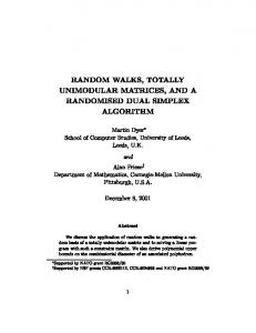
Figure 1: (Left) Bipartite graph representation, (Right) Intersection graph representation of the group structure G = {G1 = {2}, G2 = {1, 3, 4}, G3 = {2, 3, 6}, G4 = {5, 6}, G5 = {5, 7}}

5

∗∗ Figure 2: Unit norm ball of gG,∩ , for G = {{1, 2}, {2, 3}}, unit group weights d = 1.

Group sparsity

Group sparsity is an important class of structured sparsity models that arise naturally in machine learning applications (cf., [26] and the citations therein), where prior information on x\ dictates certain groups of variables to be selected or discarded together.

and the vector d ∈ RM to positive group + here corresponds ω weights. Recall that β = , and thus Hβ ≤ 0 simply s corresponds to sj ≤ wi , ∀j ∈ Gi .

A group sparsity model thus consists of a collection of potentially overlapping groups G = {G1 , · · · , GM } that cover the ground set P, where each group Gi ⊆ P is a subset of variables. A group structure construction immediately supports two compact graph representations (c.f., Figure 1).

gG,∩ (x) indeed sums up the weight of the groups intersecting with the support, since for any coefficient in the support of x the constraint Hβ ≤ 0 forces all the groups that contain this coefficient to be selected.

First, we can represent G as a bipartite graph [3], where the groups form one set, and the variables form the other. A variable i ∈ P is connected by an edge to a group Gj ∈ G iff i ∈ Gj . We denote by B ∈ {0, 1}p×M the biadjacency matrix of this bipartite graph; Bij = 1 iff i ∈ Gj , and by E ∈ {0, 1}|E|×(M +p) its edge-node incidence matrix; Eij = 1 iff the vertex j is incident to the edge ei ∈ E. Second, we can represent G as an intersection graph [3], where the vertices are the groups Gi ∈ G. Two groups Gi and Gj are connected by an edge iff Gi ∩ Gj 6= ∅. This structure makes it explicit whether groups themselves have cyclic interactions via variables, and identifies computational difficulties. 5.1

Group intersection sparsity

In group sparse models, we typically seek to express the support of x\ using only few groups. One natural penalty to consider then is the non-decreasing submodular function that sums up the weight P of the groups intersecting with the support F∩ (S) = Gi ∈G,S∩Gi 6=∅ di . The convexification of this function results in the `∞ -group lasso norm (also known as ∞-CAP penalties) [12, 27], as shown in [1]. We now show how to express this penalty as a TU penalty.

Here, H is TU, since each row of H contains at most two non-zero entries, and the entries in each row with two nonzeros sum up to zero, which is a sufficient condition for total unimodularity [17, Proposition 2.6]. Proposition 2 (Convexification). The convex envelope of gG,∩ (x) over the unit `∞ -ball is (P if x ∈ [−1, 1]p ∗∗ Gi ∈G di kxGi k∞ gG,∩ (x) = ∞ otherwise

5.2

Minimal group cover

The groups intersections penalty induces supports corresponding to the intersection of the complements of groups, while in several applications, it is desirable to explain the support of x\ as the union of groups in G. In particular, we can seek the minimal set cover of x\ : Definition 6 (Group `0 -“norm”, [3]). The group `0 “norm” computes the weight of the minimal weighted set cover of x with group weights d ∈ RM +: gG,0 (x) :=

min

ω∈{0,1}M

{dT ω : Bω ≥ 1supp(x) },

where B is the biadjacency matrix of the bipartite graph representation of G.

Definition 5 (Group intersection sparsity). gG,∩ (x) :=

min

ω∈{0,1}M

{dT ω : Hβ ≤ 0, 1supp(x) = s}

where H is the following matrix:   −I M , H 1 ( −I M , H 2  1   H :=   , H k (i, j) = 0 ··· −I M , H p

if j = k, j ∈ Gi otherwise

Note that computing the group `0 -“norm” is NP-Hard, since it corresponds to the minimum weight set cover problem. gG,0 (x) is a penalty that was previously considered in [3, 20, 11], and the latent group lasso was proposed in [20] as a potential convex surrogate for it, but it was not established as the tightest possible convexification. The group `0 -“norm” is not a submodular function, but if B is TU, it is a TU penalty, and thus is admits a tight


Proposition 5 (Convexification). The convex surrogate via Proposition 1 for gG,s (x) with M = H (i.e., the group intersection model with sparse groups) is given by ΩG,s (x) :=

X

(kxGi k∞ + |xj | − 1)+

(i,j)∈E

∗∗ Figure 3: Unit norm ball of gG,0 , for G = {{1, 2}, {2, 3}}, unit group weights d = 1.

convex relaxation. We show below that the convex envelope of the group `0 -“norm” is indeed the `∞ -latent group norm. It is worth noting that the `q -latent group lasso was also shown in [19] to be the positive homogeneous convex envelope of the `q -regularized group `0 -“norm”, i.e., of µg(x)G,0 + νkxkq . Proposition 3 (Convexification). When the group structure leads to a TU biadjacency matrix B, the convex envelope of the group `0 -“norm” over the unit `∞ -ball is ( ∗∗ gG,0 (x) =

minω∈[0,1]M {dT ω : Bω ≥ |x|} if x ∈ [−1, 1]p ∞ otherwise

for x ∈ [−1, 1]p , and ΩG,s (x) := ∞ otherwise. Note that ∗∗ ΩG,s (x) ≤ gG,s (x). By construction, the convex penalty proposed by Proposition 5 is different from the sparse group lasso in [22]. Analogous to the latent group norm, we can seek to convexify the sparsest set cover with sparsity within groups: Proposition 6 (Convexification). The convex surrogate via Proposition 1 for gG,s (x) with M = [−B, I p ] (i.e., the group `0 -“norm” with sparse groups) is given by ΩG,s (x) :=

Remark 5. One important class of group structures that leads to a TU matrix B is given by acyclic groups, as shown in [3, Lemma 2]. The induced intersection graph for such groups is acyclic, as illustrated in Figure 1. In this case, the `∞ -latent group norm is a tight relaxation. 5.3

Sparsity within groups

Both group model penalties we considered so far only induce sparsity on the group level; if a group is selected, all variables within the group are encouraged to be non-zero. In some applications, it is desirable to also enforce sparsity within groups. We thus consider a natural extension of the above two penalties, where each group is weighed by the `0 -norm of x restricted to the group. Definition 7 (Group models with sparsity within groups). gG,s (x) =

min

ω∈{0,1}M

{

M X

ωi kxGi k0 : M β ≤ 0, 1supp(x) = s}

i=1

where M here is either M = H in Definition 5 or M = [−B, I p ] in Definition 6. Unfortunately, this penalty leads to a non-TU penalty, and thus its corresponding convex surrogate given by Proposition 1 is not guaranteed to be tight. Proposition 4. Given any group structure G, gG,s (x) is not a TU penalty.

ω∈[0,1]M

X

(ωi + |xj | − 1)+ : Bω ≥ |x|}

(i,j)∈E

for x ∈ [−1, 1]p , and g(x)G,s = ∞ otherwise. 5.4

Thus, given a group structure G, one can check in polynomial time if it is TU [25] to guarantee that the `∞ -latent group lasso will be the tightest relaxation.

min {

Sparse G-group cover

In this section, we provide a more direct formulation to enforce sparsity both on the coefficients and the group level. If the true signal x\ we are seeking is a sparse signal covered by at most G groups, it would make sense to look for the sparsest signal with a G-group cover that explains the data in (2). This motivates the following natural penalty. Definition 8 (Sparse G-group cover). gG,G (x) :=

min {1T s : Bω ≥ s, 1T ω ≤ G, s = 1supp(x) }

ω∈{0,1}p

where B is the biadjacency matrix of the bipartite graph representation of G. If the actual number of active groups is not known, G would be a parameter to tune. Note that gG,G is an extension of the minimal group cover penalty (c.f., Section 5.2), where instead of looking for the signal with the smallest cover, we seek the sparsest signal that admit a cover with fewer than G groups. gG,G is a TU penalty whenever e = B is TU [17, Proposition 2.1], which is the case, B 1 for example, when B is an interval matrix. Proposition 7 (Convexification). When the group structure e the convex envelope of leads to a TU constraint matrix B, gG,G over the unit `∞ -ball is ∗∗ gG,G (x) =

min {kxk1 : Bω ≥ |x|, 1T ω ≤ G}

ω∈[0,1]M

∗∗ for x ∈ [−1, 1]p , and gG,G (x) = ∞ otherwise.


norm we studied in Section 5.1 as the convex envelope of gG,∩ (x). In this sense, gG,∩ (x) is equivalent to gT,0 (x), for the group structure GH (for unit weights).

6

Dispersive sparsity models

Figure 4: Valid selection (left), Invalid selection (right)

∗∗ Figure 5: Unit norm ball of gT,0 , GH = {{1, 2, 3}, {2}, {3}}

The resulting convex program thus combines the latent group lasso (c.f., Section 5.2) with the `1 norm and provides an alternative to the sparse group lasso in [22], for the overlapping groups case. In the supplementary material we provide a numerical illustration of its performance. 5.5

Hierarchical model

We study the hierarchical sparsity model, where the coefficients of x\ are organized over a tree T , and the non-zero coefficients form a rooted connected subtree of T (cf., Figure 4). This model is popular in image processing due to the natural structure of wavelet coefficients [13, 7, 24]. We can describe such a hierarchical model as a TU model: Definition 9 (Tree `0 -“norm”). We define the penalty encoding the hierarchical model on x as ( kxk0 if T 1supp(x) ≥ 0 gT,0 (x) := ∞ otherwise where T is the edge-node incidence matrix of the directed tree T , i.e., Tli = 1 and Tlj = −1 iff el = (i, j) is an edge in T . It encodes the constraint sparent ≥ schild for s = 1supp(x) over the tree. This is indeed a TU model since each row of T contains at most two non-zero entries that sum up to zero [17, Proposition 2.6]. Proposition 8. (Convexification) The convexification of the tree `0 -“norm” over the unit `∞ -ball is given by (P if x ∈ [−1, 1]p ∗∗ G∈GH kxG k∞ gT,0 (x) = ∞ otherwise where the groups G ∈ GH are defined as each node and all its descendants. Note that the resulting convex norm is the `∞ -hierarchical group norm [13], which is a special case of `∞ -group

The sparsity models we considered thus far encourage clustering. The implicit structure in these models is that coefficients within a group exhibit a positive, reinforcing correlation. Loosely speaking, if a coefficient within a group is important, so are the others. However, in many applications, the opposite behavior may be true. That is, sparse coefficients within a group compete against each other [28, 10, 8]. Hence, we describe models that encourage the dispersion of sparse coefficients. Here, dispersive models still inherit a known group structure G, which underlie their interactions in the opposite manner to the group models in Section 5. 6.1

Group knapsack model

One natural model for dispersiveness allows only a certain budget of coefficients, e.g., only one, to be selected in each group:  FD (S) =

 if S = ∅ 0 1 if maxG∈G |S ∩ G| ≤ 1  ∞ otherwise

Whenever the group structure forms a partition of P, [19] shows that the positive homogeneous convex envelope of the `q -regularized group knapsack model, i.e., of µFD (supp(x)) + νkxkq , is the exclusive norm in [28]. In what follows, we prove that FD (S) is a TU penalty whenever the group structure leads to a TU biadjacency matrix B of the bipartite graph representation, which includes partition structures. We establish that the `∞ exclusive lasso, is actually the tightest convex relaxation of a more relaxed version of FD (supp(x)) for any TU group structure, and not necessarily partition groups. Definition 10 (Group knapsack penalty). Given a group structure G that leads to a TU biadjacency matrix B, FD (supp(x)) can be written as the following TU penalty: gD (x) := min {ω : B T 1supp(x) ≤ ω1} ω∈{0,1}

if B T 1supp(x) ≤ 1, and gD (x) = ∞ otherwise. Note that if B is TU, B T is also TU [17, Proposition 2.1]. Groups that form a partition of P are acyclic, thus the corresponding matrix B is TU trivially (cf., Remark 5). Another important example of a TU group structure arises from the simple one-dimensional model of the neuronal signal suggested by [10]. In this model, neuronal signals are seen as a train of spike signals with some refractoriness


period ∆ ≥ 0, where the minimum distance between two non-zeros is ∆. This structure corresponds to an interval matrix B T = D, which is TU [17, Corollary 2.10]. 1 0  D=  

1 1

0

···



··· 1

1 ···

1 1 ..

0

0

0 1

0 0

··· ···

1

···

1

.

1

 0 0     1

(p−∆+1)×p

Proposition 9 (Convexification). The convex envelope of gD (x) over the unit `∞ -ball when B T is a TU matrix is given by ( maxG∈G kxG k1 if x ∈ [−1, 1]p , B T |x| ≤ 1 ∗∗ gD (x) = ∞ otherwise Notice that the convexification of gD is not exactly the exclusive lasso; it has an additional budget constraint B T |x| ≤ 1. Thus in this case, regularizing with the `q norm before convexifying lead to the loss of part of the structure. In fact, the exclusive norm is actually the convexification of a more relaxed version of gD , where the constraint ω ∈ {0, 1} is relaxed to ω ∈ Z, ω ≥ 0. 6.2

Sparse group knapsack model

In some applications, it may be desirable to seek the sparsest signal satisfying the dispersive structure. This can be achieved by incorporating sparsity into the group knapsack penalty, resulting in the following TU penalty. Definition 11 (Dispersive `0 -“norm”). Given a group structure G that leads to a TU biadjacency matrix B, we define the penalty encoding the sparse group knapsack model on x as ( kxk0 if B T 1supp(x) ≤ 1 gD,0 (x) := ∞ otherwise We can compute the convex envelope of gD,0 (x) in a similar fashion to Proposition 9. Proposition 10. (Convexification) The convexification of the dispersive `0 -“norm” over the unit `∞ -ball is given by ( kxk1 if x ∈ [−1, 1]p , B T |x| ≤ 1 ∗∗ gD,0 (x) = ∞ otherwise It is worth mentioning that regularizing with the `q -norm here loses the underlying dispersive structure. In fact, the positively homogeneous convex envelope of µgD,0 (x) + λkxkq is given by the dual (cf., Section 3.3) of Ω∗q (y) =

max

s∈{0,1}p ,s6=0,B T s≤1

ky supp(s) kq (1T s)1/q

∗∗ ∗∗ Figure 6: gD,0 (x) ≤ 1 (left) gD,0 (x) ≤ 1.5 (middle) ∗∗ gD,0 (x) ≤ 2 (right) for G = {{1, 2}, {2, 3}}

which is simply the `1 -norm. To see this, note that P |yi |q |S|kykq∞ Ω∗a (y)q = kyk∞ , since i∈S ≤ , ∀S ⊆ P |S| |S| which is achieved with equality by choosing the vector s having ones where y is maximal, and zeros elsewhere. Note that this vector satisfies B T s ≤ 1. As a result, the regularized convexification boils down to the `1 -norm, since Ωq (x) = supΩ∗q (y)≤1 xT y = kxk1 , while the direct convexification is not even a norm (cf., Figure 6). We illustrate the effect of this loss of structure via a numerical example in Section 7. 6.3

Graph dispersiveness

In this section, we illustrate that our framework is not limited to linear costs, by considering a pairwise dispersive model. We assume that the parameter structure is encoded on a known graph G(P, E), where coefficients connected by an edge are discouraged from being on simultaneously. Definition 12 (Pairwise dispersive penalty). Given a graph G(P, E) with a TU edge-node incidence matrix E G (e.g., bipartite graph), we define the penalty encoding the pairwise dispersive model as X gG,D (x) = si sj where s = 1supp(x) (i,j)∈E

Note that this function is not submodular; in fact, gG,D (x) is a supermodular function. Proposition 11 (Convexification). The convex envelope of gG,D (x) over the unit `∞ -ball is (P p ∗∗ (i,j)∈E (|xi | + |xj | − 1)+ if x ∈ [−1, 1] gG,D (x) = ∞ otherwise Proof. We use the linearization trick employed in [15] to reduce gG,D (x) to a TU penalty. Let s = 1supp(x) , gG,D (x) =

X

si sj

(i,j)∈E

= =

min

z∈{0,1}|E|

min

z∈{0,1}|E|

{

X

zij : zij ≥ si + sj − 1}

(i,j)∈E

{

X

(i,j)∈E

zij : E G s ≤ z − 1}

A totally unimodular view of structured sparsity 1

1

1

0.8

0.8

0.8

0.6

0.6

0.6

0.4

0.4

0.4

0.2

0.2

0 0

50

100

150

200

0 0

\

x

∗∗ ∗∗ Figure 7: gG,D (x) = 0 (left) gG,D (x) ≤ 1 (right) for E = {{1, 2}, {2, 3}} (chain graph)

? Error: kbxkx−x? k 2k 2

0.8

150

200

xBP solution kx\ −xBP k2 kx\ k2

= .200

0 0

50

100

150

200

xDBP solution kx\ −xDBP k2 kx\ k2

= .067

0.6

fairness. We use an interior point method to obtain high accuracy solutions to each formulation.

0.4

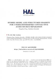
Figure 8 shows that DBP outperforms BP as we vary the number of measurements. Note that the number of measurements needed to achieve a certain error is expected to be lower for DBP than BP, as theoretically characterized in [10]. Hence, by changing the objective in the convexification, Figure 11 reinforces the message that we can lose the tightness in capturing certain structured sparsity models.

0.2

0.1

0.2

0.3

0.4

n/p

Figure 8: Recovery error of BP and DBP Now we can apply Proposition 1 to compute the convex envelope. The resulting convexification is again not a norm (c.f., Figure 7).

7

100

Figure 9: Example spike train recovery when n = 0.18p. The DBP formulation (right) shrinks the competing sparse coefficients within the ∆ intervals, resulting in a better reconstruction overall sampling regimes than BP (middle).

BP DBP

1

relative errors:

0.2

50

Numerical illustration

In this section, we show the impact of convexifying two different simplicity objectives under the same dispersive structural assumptions. Specifically, we consider minimizing the convex envelope of the `q -regularized dispersive `0 “norm” [19] versus its convex envelope without regularization over the unit `∞ -ball in Section 6.2. To produce the recovery results in Figure 8, we generate a train of spikes of equal value for x\ in dimensions p = 200 with a refractoriness of ∆ = 25 (cf., Figure 11). We then recover x\ from its compressive measurements y = Ax\ + w, where the noise w is also a sparse vector, with 15 non-zero Gaussian values of variance σ = 0.01 and A is a random column normalized Gaussian matrix. Since the noise is sparse, we encode the data via ky − Axk1 ≤ kwk1 using the true `1 norm of the noise. We produce the data randomly 20 times and report the averaged results.

8

Conclusions

We have provided a principled recipe for designing convex formulations that jointly express models of simplicity and structure for sparse recovery, that promotes clustering or dispersiveness. The main hallmark of our approach is its pithiness in generating the prevalent convex structured sparse formulations and in explaining their tightness. Our key idea relies on expressing sparsity structures via simple linear inequalities over the support of the unknown parameters and their corresponding latent group indicators. By recognizing the totally unimodularity of the underlying constraint matrices, we can tractably compute the biconjugation of the corresponding combinatorial simplicity objective subject to structure, and perform tractable recovery using standard optimization techniques. Acknowledgements This work was supported in part by the European Commission under Grant MIRG-268398, ERC Future Proof, SNF 200021- 132548, SNF 200021-146750 and SNF CRSII2147633.

\

x k2 Figure 8 measures the relative recovery error with kxkx−ˆ , \k 2 as we vary the number of compressive measurements. The regularized convexification simply leads to Basis Pursuit formulation (BP), while the TU convexification results in the addition of a budget constraint B T |x| ≤ 1 to the BP formulation, as described in Section 6.2. We refer to the resulting criteria as Dispersive Basis Pursuit (DBP). Since the DBP criteria uses the fact that x\ lies in the unit `∞ ball, we include this constraint in the BP formulation for

A

Numerical illustration of Sparse G-group cover’s performance

In this section, we compare the performance of minimizing ∗∗ the TU relaxation gG,G of the proposed Sparse G-group cover (c.f., Section 5.4) in problem (2), which we will call Sparse latent group lasso (SLGL), with Basis pursuit (BP) and Sparse group Lasso (SGL). Recall the SGL criteria is


sition 1 in the main text, to compute its convex envelope: ��

∗∗ gG,∩ (x) =

{dT ω : Hβ ≤ 0, |x| ≤ s} ω = min {dT ω : H ≤ 0} |x| ω∈[0,1]M X di kxGi k∞ (since wi∗ = kxG k∞ ) = min

s∈[0,1]p ,ω∈[0,1]M

Gi ∈G ∗∗ for x ∈ [−1, 1]p , gG,∩ (x) = ∞ otherwise.

Figure 10: Recovery error of SLGL, SGL, and BP

C (1−α)

P

p |G|kxG kq +αkxG k1 , with q = 2 in [22]. We G∈G

compare also against SGL∞ where we set q = ∞, which is better suited for signals with equal valued non-zero coefficients. We generate a sparse signal x\ in dimensions p = 200, covered by G = 5 groups, randomly chosen from the M = 29 groups. The groups generated are interval groups, of equal size of 10 coefficients, and with an overlap of 3 coefficients between each two consecutive groups. The true signal x\ has 3 non-zero coefficients (all set to one) in each of its 5 active groups (cf., Figure 11). Note that these groups lead a TU group structure G, so the TU relaxation in this case is tight. We recover x\ from its compressive measurements y = Ax\ + w, where the noise w is a random Gaussian vector of variance σ = 0.01 and A is a random column normalized Gaussian matrix. We encode the data via ky − Axk2 ≤ kwk2 using the true `2 -norm of the noise. We produce the data randomly 10 times and report the averaged results. Figure 10 measures the relative recovery error with kx\ −ˆ xk2 , as we vary the number of compressive measurekx\ k2 ments. Since the SLGL criteria uses the fact that x\ lies in the unit `∞ -ball, we include this constraint in the all the other formulations for fairness. Since the true signal exhibit strong overall sparsity we use α = 0.95 in SGL as suggested in [22] (we tried several values of α, and this seemed to give the best results for SGL). We use an interior point method to obtain high accuracy solutions to each formulation. Figure 8 shows that SLGL outperforms the other criterias as we vary the number of measurements.

B

Proof of Proposition 2

∗∗ gG,∩ (x)

=

Gi ∈G

∞

Proposition (Convexification). When the group structure leads to a TU biadjacency matrix B, the convex envelope of the group `0 -“norm” over the unit `∞ -ball is ( ∗∗ gG,0 (x)

=

∗∗ gG,0 (x) =

=

if x ∈ [−1, 1]p otherwise

Proof. Since gG,∩ (x) is a TU-penalty, we can use Propo-

min

s ∈ [0, 1]p ω ∈ [0, 1]M

{dT ω : Bω ≥ s, |x| ≤ s}

min {dT ω : Bω ≥ |x|}

ω∈[0,1]M

∗∗ for x ∈ [−1, 1]p , gG,0 (x) = ∞ otherwise.

D


Proposition. Given any group structure G, gG,s (x) is not a TU penalty. Proof. Let G(G ∪ P, E) denote the bipartite graph representation of the group structure G. We use the linearization trick employed in [15] to reduce gG,s (x) to an integer program. For conciseness, we consider gG,s (s) only for binary vectors s ∈ {0, 1}p , since gG,s (x) = gG,s (1supp(x) ).

= =

di kxGi k∞

minω∈[0,1]M {dT ω : Bω ≥ |x|} if x ∈ [−1, 1]p ∞ otherwise

Proof. Note that gG,0 (x) can be written in the form given in Definition 4 with M = [−B, I p ] and c = 0. Thus, when B is TU, so is M [17, Proposition 2.1], and thus we can use Proposition 1 in the main text, to compute its convex envelope:

gG,s (s) =

Proposition (Convexification). The convex envelope of gG,∩ (x) over the unit `∞ -ball is (P


min

ω∈{0,1}M

min

ω∈{0,1}M

{

ω∈{0,1}M

ωi ksGi k0 : M β ≤ 0}

i=1

{

X

ωi sj : M β ≤ 0}

(i,j)∈E

min {

z∈{0,1}|E|

M X

X

zij : M β ≤ 0, Eβ ≤ z + 1}

(i,j)∈E

Recall that E is the edge-node incidence matrix of G(G ∪ P, E). The constraint Eβ ≤ z − 1 corresponds to zij ≥ ωi + sj − 1, ∀(i, j) ∈ E. Although both matrices M and E


1

1

1

1

1

0.8

0.8

0.8

0.8

0.8

0.6

0.6

0.6

0.6

0.6

0.4

0.4

0.4

0.4

0.4

0.2

0.2

0.2

0.2

0 0

50

100

150

200

0 0

x\ relative errors:

50

100

150

200

xBP solution kx\ −xBP k2 kx\ k2

= .128

0 0

50

100

150

200

xSGL solution kx\ −xSGL k2 kx\ k2

0 0

0.2

50

100

150

0 0

200

50

xSGL∞ solution

= .181

kx\ −xSGL k ∞ 2 kx\ k2

100

150

200

xSLGL solution

= .085

kx\ −xSLGL k2 kx\ k2

= .058

Figure 11: Recovery for n = 0.25p, s = 15, p = 200, G = 5 out of M = 29 groups. M is not TU. To see E this, let us first focus on the case where M = [−B, I p ]. f = are TU, their concatenation M

Given any coefficient i ∈ P covered by at least one group Gi , we denote the corresponding edge in the bipartite graph by ej = (i, M + i), which corresponds to the j th row f i,i = of E. This translates into having the entries M f i,M +i = 1, M f p+j,i = 1, and M f p+j,M +i = 1. The −1, M determinant of the submatrix resulting from these entries is −2, which contradicts the definition of TU (cf., Def. 4). It f is TU iff G = {∅}. follows then that M A similar argument holds for M = H.

E


Proposition (Convexification). The convex surrogate via Proposition 1 in the main text, for gG,s (x) with M = H (i.e., the group intersection model with sparse groups) is given by X ΩG,s (x) := (kxGi k∞ + |xj | − 1)+

for x ∈ [−1, 1]p , ΩG,s (x) = ∞ otherwise. Proof. For x ∈ [−1, 1]p , ΩG,s (x) =min {

X

zij : Bω ≥ s, Eβ ≤ z + 1, |x| ≤ s}

ω∈[0,1]M (i,j)∈E z∈[0,1]|E|

=

min {

ω∈[0,1]M

X

(ωi + |xj | − 1)+ : Bω ≥ |x|}

(i,j)∈E

∗ since s∗ = |x|, and zij = (ωi + s∗j − 1)+ .

G


Proposition. (Convexification) The convexification of the tree `0 -“norm” over the unit `∞ -ball is given by (P if x ∈ [−1, 1]p ∗∗ G∈GH kxG k∞ gT,0 (x) = ∞ otherwise Proof. Since this is a TU-penalty we can use Proposition 1 in the main text, to compute its convex envelope: ∗∗ gT,0 (x) = min p {1T s : T s ≥ 0, |x| ≤ s} s∈[0,1] X ? = kxG k∞

(i,j)∈E p

for x ∈ [−1, 1] , and, ΩG,s (x) := ∞ otherwise. Note that ∗∗ ΩG,s (x) ≤ gG,s (x).

G∈GH p

for x ∈ [−1, 1] , ∞ otherwise, and where the groups G ∈ GH are defined as each node and all its descendants. Proof. For x ∈ [−1, 1] , (?) holds since any feasible s should satisfy s ≥ |x| and X ΩG,s (x) = min { zij : Hβ ≤ 0, Eβ ≤ z + 1, |x| ≤ s} sparent ≥ schild , so starting from the leaves, each leaf satω∈[0,1]M (i,j)∈E isfies si ≥ |xi |, and since we are looking to minimize the z∈[0,1]|E| X sum of si ’s, we simply set si = xi . For a node i with two = (kxGi k∞ + |xj | − 1)+ children j, k as leaves, it will satisfy si ≥ |xi |, |sj |, |sk |, (i,j)∈E thus si = max{|xi |, |xj |, |xk |}, and so on. Thus, si = ∗ since ωi∗ = kxGi k∞ , s∗ = |x|, and zij = (ωi∗ + s∗j − 1)+ . max{k is a descendant of i or i itself} |xk | p

F


Proposition (Convexification). The convex surrogate given by Proposition 1 in the main text, for gG,s (x) with M = [−B, I p ] (i.e., the group `0 -“norm” with sparse groups) is given by X ΩG,s (x) := min { (ωi + |xj | − 1)+ : Bω ≥ |x|} ω∈[0,1]M

(i,j)∈E

H


Proposition (Convexification). The convex envelope of gD (x) over the unit `∞ -ball when B T is a TU matrix is given by ( maxG∈G kxG k1 if x ∈ [−1, 1]p , B T |x| ≤ 1 ∗∗ gD (x) = ∞ otherwise


Proof. Since this is a TU penalty we can use Proposition 1 in the main text, to compute its convex envelope: ( T

min ω∈[0,1] {ω : B s ≤ ω1, |x| ≤ s} if x feasible

∗∗ gD (x) =

s∈[0,1]p

∞

( =

I

otherwise

kB T |x|k∞ ∞

if x ∈ [−1, 1]p , B T |x| ≤ 1 otherwise


Proposition (Convexification). The convex envelope of gG,D (x) over the unit `∞ -ball is (P if x ∈ [−1, 1]p ∗∗ (i,j)∈E (|xi | + |xj | − 1)+ gG,D (x) = ∞ otherwise Proof. We use the linearization trick employed in [15] to reduce gG,D (x) to a TU penalty. Let s = 1supp(x) , X gG,D (x) = si sj (i,j)∈E

= =

min

z∈{0,1}|E|

min

z∈{0,1}|E|

{

X

zij : zij ≥ si + sj − 1}

(i,j)∈E

{

X

zij : E G s ≤ z − 1}

(i,j)∈E

[5] V. Chandrasekaran, B. Recht, P.A. Parrilo, and A.S. Willsky. The convex geometry of linear inverse problems. Foundations of Computational Mathematics, 12:805–849, 2012. [6] P. Kothari D. Chakrabarty, P. Jain. Provable submodular minimization using wolfe’s algorithm. NIPS, 2014. [7] Marco F Duarte, Michael B Wakin, and Richard G Baraniuk. Wavelet-domain compressive signal reconstruction using a hidden markov tree model. In Acoustics, Speech and Signal Processing, 2008. ICASSP 2008. IEEE International Conference on, pages 5137–5140. IEEE, 2008. [8] W Gerstner and W. Kistler. Spiking neuron models: Single neurons, populations, plasticity. Cambridge university press, 2002. [9] FR Giles and William R Pulleyblank. Total dual integrality and integer polyhedra. Linear algebra and its applications, 25:191–196, 1979. [10] C. Hegde, M. Duarte, and V. Cevher. Compressive sensing recovery of spike trains using a structured sparsity model. In SPARS’09-Signal Processing with Adaptive Sparse Structured Representations, 2009. [11] J. Huang, T. Zhang, and D. Metaxas. Learning with structured sparsity. The Journal of Machine Learning Research, 12:3371–3412, 2011.

Now we can apply Proposition 1 in the main text, to compute the convex envelope:

[12] R. Jenatton, J.-Y. Audibert, and F. Bach. Structured variable selection with sparsity-inducing norms. ∗∗ gG,D (x) = min { zij : E G s ≤ z − 1, |x| ≤ s} Journal of Machine Learning Research, 12:2777– s∈[0,1]p ,z∈[0,1]|E| (i,j)∈E 2824, 2011. X X

(|xi | + |xj | − 1)+

=

(i,j)∈E ∗

(s =

∗ x, zij

=

(s∗i

+

s∗j

− 1)+ )

∗∗ for x ∈ [−1, 1]p , gG,D (x) = ∞ otherwise.

References [1] F. Bach. Structured sparsity-inducing norms through submodular functions. In NIPS, pages 118–126, 2010. [2] F. Bach. Learning with submodular functions: A convex optimization perspective. arXiv preprint arXiv:1111.6453, 2011.

[13] R. Jenatton, J. Mairal, G. Obozinski, and F. Bach. Proximal methods for hierarchical sparse coding. Journal of Machine Learning Reasearch, 12:2297– 2334, 2011. [14] Vladimir Jojic, Suchi Saria, and Daphne Koller. Convex envelopes of complexity controlling penalties: the case against premature envelopment. In International Conference on Artificial Intelligence and Statistics, pages 399–406, 2011. [15] Marcin Kamiński. Quadratic programming on graphs without long odd cycles. 2008.

[3] L. Baldassarre, N. Bhan, V. Cevher, and A. Kyrillidis. Group-sparse model selection: Hardness and relaxations. arXiv preprint arXiv:1303.3207, 2013.

[16] A. Kyrillidis and V. Cevher. Combinatorial selection and least absolute shrinkage via the clash algorithm. In Information Theory Proceedings (ISIT), 2012 IEEE International Symposium on, pages 2216– 2220. Ieee, 2012.

[4] R.G. Baraniuk, V. Cevher, M.F. Duarte, and C. Hegde. Model-based compressive sensing. Information Theory, IEEE Transactions on, 56(4):1982–2001, 2010.

[17] George L Nemhauser and Laurence A Wolsey. Integer and combinatorial optimization, volume 18. Wiley New York, 1999.


[18] B. Nirav, L. Baldassarre, and V. Cevher. Tractability of interpretability via selection of group-sparse models. In Information Theory (ISIT), 2013 IEEE International Symposium on, 2013. [19] G. Obozinski and F. Bach. ation for combinatorial penalties. arXiv:1205.1240, 2012.

Convex relaxarXiv preprint

[20] G. Obozinski, L. Jacob, and J.P. Vert. Group lasso with overlaps: The latent group lasso approach. arXiv preprint arXiv:1110.0413, 2011. [21] C Seshadhri and Jan Vondrák. Is submodularity testable? Algorithmica, 69(1):1–25, 2014. [22] Noah Simon, Jerome Friedman, Trevor Hastie, and Robert Tibshirani. A sparse-group lasso. Journal of Computational and Graphical Statistics, 22(2):231– 245, 2013. [23] Maurice Sion et al. On general minimax theorems. Pacific J. Math, 8(1):171–176, 1958. [24] Akshay Soni and Jarvis Haupt. Efficient adaptive compressive sensing using sparse hierarchical learned dictionaries. In Signals, Systems and Computers (ASILOMAR), 2011 Conference Record of the Forty Fifth Asilomar Conference on, pages 1250–1254. IEEE, 2011. [25] Klaus Truemper. Alpha-balanced graphs and matrices and GF(3)-representability of matroids. Journal of Combinatorial Theory, Series B, 32(2):112–139, 1982. [26] Martin J Wainwright. Structured regularizers for high-dimensional problems: Statistical and computational issues. Annual Review of Statistics and Its Application, 1:233–253, 2014. [27] Peng Zhao, Guilherme Rocha, and Bin Yu. Grouped and hierarchical model selection through composite absolute penalties. Department of Statistics, UC Berkeley, Tech. Rep, 703, 2006. [28] Y. Zhou, R. Jin, and S. Hoi. Exclusive lasso for multitask feature selection. In International Conference on Artificial Intelligence and Statistics, pages 988–995, 2010.