In proceedings of the International Conference on Artificial Neural Networks and Genetic Algorithms, pp. 41-44, 1995.
A TRANSFORMATION FOR IMPLEMENTING EFFICIENT DYNAMIC BACKPROPAGATION NEURAL NETWORKS George L. Rudolph and Tony R. Martinez Computer Science Department, Brigham Young University, Provo, Utah 84602 e-mail:
[email protected],
[email protected] Abstract Most Artificial Neural Networks (ANNs) have a fixed topology during learning, and often suffer from a number of short-comings as a result. Variations of ANNs that use dynamic topologies have shown ability to overcome many of these problems. This paper introduces Location-Independent Transformations (LITs) as a general strategy for implementing distributed feedforward networks that use dynamic topologies (dynamic ANNs) efficiently in parallel hardware. A LIT creates a set of location-independent nodes, where each node computes its part of the network output independent of other nodes, using local information. This type of transformation allows efficient support for adding and deleting nodes dynamically during learning. In particular, this paper presents an LIT for standard Backpropagation with two layers of weights, and shows how dynamic extensions to Backpropagation can be supported. 1. INTRODUCTION This paper proposes a strategy for implementing standard and dynamic backpropagation neural networks in parallel hardware: LIT BP (Location-Independent Transformation for Backpropagation Networks). LIT BP is part of an effort to develop a general strategy (called LIT) for implementing ANNs. This strategy supports general classes of ANNs and efficiently supports ANNs with dynamic topologies [5-7]. A dynamic topology is one which allows adding and deleting both nodes and weighted connections during learning. Hardware support for ANNs is important for handling large, complex problems in real time. Learning times for complex applications can exceed tolerable limits using conventional computing schemes. Furthermore, hardware is becoming cheaper and easier to design. LIT overcomes several weaknesses of current hardware implementation methods. Most ANNs use static topologies—the topology is fixed initially, and remains the same throughout learning. ANNs with static topologies often suffer from the following shortcomings: 1) sensitivity to user-supplied parameters—learning rate(s), momentum, etc., 2) local error minima during learning, and 3) there is no mechanism for deciding on an effective initial topology (number of nodes, number of layers, etc.) Current research is demonstrating the use of dynamic topologies in overcoming these problems [1], [3], [4]. Early ANN hardware implementations were model-specific, and are intended to support only static topologies. More recent neurocomputer systems have specialized neural hardware, and seek to support more general classes of ANNs [2]. Although some neurocomputers could potentially support dynamic topologies more directly in hardware, rather than in software, they currently do not. Of course, general parallel machines, like the Connection Machine, can simulate the desired dynamics in software, but these machines are not optimized for neural computation. LIT supports general classes of ANNs and dynamic topologies in an efficient parallel hardware implementation. LIT redesigns the original network into a hierarchical, parallel network in which each node
† This research is funded by grants from Novell Inc. and Word Perfect Corp.
2
contains enough information locally to compute its part of the network output, independent of any other node. A network whose nodes have this property is said to be location-independent. The nodes also are location-independent—regardless of the physical location of any node in the network, the relative order in which they compute results, or the order in which those results are gathered, the individual computations are the same, and the network output is the same. Furthermore, because a node’s information is local, adding or deleting nodes from the network can be done without affecting any other nodes. Thus, location-independence allows efficient support for dynamic topologies. A prototype VLSI chip set has been fabricated as proof-ofconcept of the overall LIT strategy [8]. This paper presents the transformation for standard backpropagation (BP) networks with a single hidden layer, and shows how dynamic extensions to BP can be supported—the same basic transformation applies to networks with an arbitrary number of layers. Many dynamic extensions to BP have been proposed in the literature. Although any of these can be supported by LIT, one algorithm that allows addition and deletion of both nodes and weights [3] is chosen as an example for this paper. Section 2 discusses the mapping from an original (either standard or extended) BP network to a transformed (LIT BP) network. Section 3 gives the algorithms for execution and learning as adapted to LIT, demonstrating the equivalence of the original and transformed networks. For brevity, the steps required for the dynamic topology have been included with the standard BP algorithm, rather than described separately. Section 4 is the conclusion. 2. CONSTRUCTION OF A BP NETWORK In this paper, the term Control Unit refers to a mechanism that broadcasts inputs to a network, and reads the results from the network. The term original refers to a network before it is transformed, and the term transformed refers to a network after it has been transformed. These terms apply similarly to the nodes as well. The number of layers refers to the number of weight layers. LIT is a two-step process: 1. Construct a set of location-independent nodes based on the original model. 2. Embed the nodes in a tree. The original BP network has a distributed internal representation of learned information. Furthermore, the model requires an efficient backward phase of learning as well as forward. The key issues for transforming the BP network are to localize enough information at a node to satisfy location-independence and allow for efficient backpropagation, while essentially preserving the distributed character of the original model. A node structure that meets these goals is given below. A binary tree topology is used for parallelism and communication in the transformed network, in this paper. Trees and other hierachical topologies allow adding or deleting nodes with time logarithmic in the number of hidden nodes in the original BP network. The connectivity among nodes in the transformed network does not explode because each node is connected to one parent and zero to two children. The algorithms for the transformed network show explicitly how communication can take place. The heart of a transformation is the construction step: It defines the mapping between the original network and the set of LI-nodes, which in turn affects how the behavior of the original network is modeled in the transformed network. The original BP equations and structures reveal a symmetry both in the information used for computation, and in the behavior during forward and backpropagation phases. The construction given here reflects that symmetry, as well as achieving the goals of LIT.
3
1
1
2
3
4
5
2
4
3
5
6
2 6
5 3
1. Transform the ANN
4
1
2. Embed the LI-nodes in a tree
Figure 2. Transforming a 2-layer BP Network. Input
x1
Output O
u
w
1j
u
2j
w
Oj 2
j2
xn un j
wj p
execution mode & forward phase of learning
Oj p
Output δw
uj1
wj 1
uj2
wj 2
j
σ( n e t )
x2
j1
j1
Input
u jn
δu
1
δw
2
j
wj p
δw
3
backpropagation phase of learning
Figure 3. A Node in the Transformed BP Network Figure 2 shows an original 2-layer BP network transformed to a LIT network with six nodes. There is one node in the transformed network corresponding to each original hidden node, plus one bias node. Figure 3 shows a general transformed BP node in detail. A transformed BP node (except the bias node) stores two vectors (layers) of weights—one on inputs (hereafter uj ) and one on outputs (hereafter wj). Each element, uij or wjk, of these vectors corresponds to a weight connected to the respective original hidden node. The original node 2, in figure 2, has four weights on inputs, and three weights on outputs. The transformed node 2 has four weights in uj and three weights in wj. Each transformed node also stores a bias value θj, which corresponds to the bias value in the respective original hidden node. For purposes of learning, θj can be treated as a component of uj . The bias node is like the other transformed nodes, with some exceptions. It needs no uj because its activation is always 1. The elements of its wj each correspond to one of the biases from the original output nodes. It has no additional bias values of its own. In all other respects, the bias node behaves like the other transformed nodes. The reason each node stores two weight vectors has to do with backpropagation learning. The computation of δ error values at an original hidden node requires access to the weight values connected to that node from the subsequent layer. This computation is thus localized by storing the needed weights at each node. This difference in structure causes some differences in
4
behavior between the original and transformed networks, though they remain quite similar. These differences are highlighted here—formal descriptions of the algorithms for the transformed network are given below in sections 3.1 and 3.2. During execution, each transformed node computes a vector of output values O j as follows: Each node recieves the input vector X and performs the sum-of-products with uj , and θj is added, to produce netj . Each component of wj is then multiplied by f(netj ) to produce Oj . The corresponding elements of each vector from all the nodes are summed together to produce a single vector of activation values. This summation is accomplished in the transformed network as each node sums its vector with those of its children, and sends the result to its parent. The parent of the root node is the Control Unit. The final output of the network is computed by applying the sigmoid function f to each element of this activation vector. Each element of the final output corresponds to one of the output nodes in the original network. As the root node sends its result to the Control Unit, the sigmoid function is applied to each element, thus the final output is held at the Control Unit. During learning, the error values for the second layer of weights (output layer in the original) are calculated at the end of the forward phase, as given in the algorithm below. The resulting vector of error values is broadcast to all the nodes. This vector is used at each transformed node to compute weight changes for the second layer of weights (including the bias node) and the δ value for the first layer of weights just as in the original network. Weight changes for the first layer of weights are computed, also as in the original. The preceeding discussion shows how the standard BP model is supported. This paragraph describes the dynamic extension to learning. The dynamic BP algorithm of [3] allows adding and deleting hidden nodes, but not input or output nodes (original network). Node addition is accomplished through probabilistic node division. The probability that a particular node will divide is a function of the global time since any node last divided, how much this node’s error corrections have oscillated over the last epoch of training, and a probability threshold value. A node which oscillates wildly will eventually divide so that one node covers one hyperplane, and one node covers the other. Node deletion is accomplished through probabilistic weight deletion. A node self-deletes whenever all the weights in uj are 0, or when all the weights in wj are 0. This is a probabilistic event, since each weight computes a probability that it will set itself to 0 after each epoch of learning. This probability is a function of the global time since the last weight was deleted in the network and how much the weight has contributed correctly to its node’s overall activity in the last epoch. The learning algorithm below includes the steps of the dynamic algorithm based on [3], but the equations and further details are not included for reasons of space. More detail is available in [3] and [7]. 3. ALGORITHMS The following definitions and equations describe execution mode and learning for the 2layer LIT BP. They are essentially the original equations, but altered to show the behavior of the LIT model. The learning algorithm also includes steps for the dynamic extension based on [3]. The main steps of the respective algorithms are in italics. The sub-steps (1.1, 2.1, etcetera) specify the details of how the LIT network accomplishes these steps. 3.1 Execution Algorithm q n m
number of weight layers in the original network. q = 2. number of nodes in the original input layer, size of uj . number of nodes in the original hidden layer, number of nodes in the transformed
5
p a Oj Oj netj f X xi uj u ij ojk wj w jk Y yk Z zk
network. number of nodes in the original output layer, size of wj. real-valued number, it will be either netj or yk. output vector of new node j. intermediate activation value for new node j, it corresponds to Oj for an original node j. real-valued sum of the inputs to node j [equation (4)]. sigmoid function. pattern clamped on inputs, has size n. ith real-valued component of X. vector of weights on inputs in a new node j, has size n. real-valued ith component of uj . It corresponds in the original network to the weight from input node i to hidden node j. real-valued kth component of Oj . It corresponds in the original network to the weight from hidden node j to output node k, multiplied by the original Oj. vector of weights on output in a new node j, has size p. real-valued kth component of wj. It corresponds in the original network to the weight from hidden node j to output node k. vector of intermediate activation values, the sum of all Oj. real-valued kth component of Y. It corresponds in the original network to the netj of output node k. vector of network output values. real-valued (always between 0 and 1)kth component of Z. It corresponds in the original network to the output Ok of output node k. 1 1+e-a Oj = f(netj )
f(a) =
(1) (2)
n
netj = ∑ xiuij + θj
(3)
ojk = Oj wjk
(4)
i=1
m
yk = ∑ojk
(5)
zk = f(yk)
(6)
j=1
The algorithm is as follows: (1)
Clamp an input pattern on the input nodes. 1.1 Broadcast input vector X to the nodes. (2) Each node takes the sigmoid of the sum-of-products of its weights and inputs. 2.1 Each node computes its netj and then computes Oj . Oj for the bias node is 1. 2.2 Each node's weight vector wj is multiplied by its (scalar) O j to produce its output vector Oj . 2.3 Each node computes the vector sum of its Oj with the result from each child, and the sum (a vector) is sent to its parent. (The Control Unit is the parent of the root node.) The result is the vector Y. (3) Wait until the activation values on the output nodes are valid. 3.1 Y is sent (through the sigmoid pipe) to the Control Unit. The result Z is the output
6
of the network. 3.2 Learning Algorithm Below are additional definitions and equations that describe the learning mode for the LIT BP. The forward phase of learning is almost identical to execution mode, and so follows the equations given above.
α weight change momentum constant. δw vector of error values for all wj . It has size p. δwk real-valued jth component of δw. It corresponds in the original network to δk for output node k. δuj real-valued error value for uj in node j. It corresponds in the original network to δj for hidden node j. T vector of target values for the current pattern being presented. It has size p. tk target value for zk. It corresponds in the original network to the target value for Ok for output node k. psse pattern sum-squared error for the current pattern being presented. tsse total sum-squared error over all patterns in the current learning epoch. ecrit maximum error tolerance for learning. s number of patterns in the training set (epoch). r simple index, used to avoid confusion with i, j, k, etc. c current training cycle number. η a real-valued learning constant. f '(a) =
∂f (a)
= f(a)(1-f(a))
(7)
∆wjk (c)= ηOjδwk+α∆wjk(c-1) ∆uij (c)= ηxiδuj +α∆uij(c-1) δwk = (tk-zk)f '(yk)
(8) (9)
δuj = (
∂a
p
∑ (δwkwjk))f '(Oj)
(10)
k=1
s
tsse =
∑ psser
(11)
r =1 p
psser =
∑ δ wk 2
(12)
k =1
As with the execution algorithm above, the main steps of the learning algorithm are in italics, and the sub-steps give the details of how LIT accomplishes each step. The learning algorithm is as follows: Until Convergence (tsse < ecrit at the end of an epoch) (1) Present a training pattern to the network 1.1 The forward phase of learning—this is same as execution above, up to (and including) step 2.3.
7
Calculate the error δ of the output units (T - O) 2.1 As each yk is sent to the Control Unit, the following occurs: 2.1.1 zk is computed and received by the Control Unit. 2.1.2 zk and tk are used to compute δ wk, received which isby the Control Unit. 2.1.3 δwk is used to compute δwk2 . 2.1.4 Each δwk2 is summed with the value of psse so far. (3) For each hidden layer Calculateδj using δk from the subsequent layer 3.1 The vector δw is broadcast to the nodes. 3.2 Calculate δuj . (4) Update the weights 4.1 Calculate ∆wjk and ∆uij. 4.2 Change the weights. (5) Update tsse (6) Perform probabilistic weight deletion 6.1 Each weight computes a probability of self-deletion in the range 0-1. 6.2 Each weight generates a random value in the range 0-1. 6.3 If the probability is greater than the random value, then the weight is deleted. (7) Perform node deletion on the hidden nodes (the number of input and output nodes remains fixed) 7.1 If uj =0, or wj =0, then node j self-deletes. 7.2 In the case that u j =0, and the bias θ j ≠0, then adjust the biases of the remaining nodes to compensate. (8) Check for node addition (by probabilistic node division). 8.1 Each node computes a probability of dividing, in the range 0-1. 8.2 Each weight generates a random value in the range 0-1. 8.3 If the probability is less than the random value, then the node does not divide—skip step 9. (9) Do node division (only if at least one node divides) 9.1 Two descendant nodes are created from the node: The uj for both remain the same as the parent, but wj are chnged so that one node covers one hyperplane and the other node covers the other hyperplane. (2)
end Step 5 may actually be computed any time after the end of step 2—independent of steps 3 or 4. Most algorithms assume that psse and tsse can be maintained, but give no explicit mechanism for doing so—LIT provides a mechanism. Conceptually, step 9 could be done at the end of step 8. However, for algorithmic purposes, it is more convenient to check for the possibility of node division separate from actually performing node division. Node division is potentially the most expensive of all steps in terms of complexity and performance. However, it is important to realize that node division is a rare event in the operation of the network; when it does occur, it is highly unlikely to tax the resources of the network—particularly large networks. First, only highly unstable nodes have high probabilities of dividing. Second, as training time increases and the network becomes more stable, it is less likely for any particular node to become unstable, and correspondingly more remote that even a few nodes will simultaneously divide.
8
[7] shows that complexity of both learning and execution algorithms is O(n+p+logm) for a single pattern, where n is the number of inputs, p is the number of outputs, and m is the number of hidden nodes in the original network. 4. CONCLUSION ANNs that use a static topology, i.e. a topology that remains fixed throughout learning, suffer from a number of short-comings. Current research is demonstrating the use of dynamic topologies in overcoming some of these problems. The Location-Independent Transformation (LIT) is a general strategy for implementing variations of ANNs that use dynamic topologies during learning. This paper introduced ideas for LITs for static and dynamic feedforward, distributed neural networks. An LIT with associated execution and learning algorithms for backpropagation were formally defined, as an example. Current work includes the following: • LITs for other ANNs, aside from those for which transformations have been developed. • VLSI design and fabrication of LIT models. REFERENCES [1]
[2]
[3]
[4] [5]
[6] [7]
[8]
Fahlmann, Scott, C. Lebiere. The Cascade-Correlation Learning Architechture. in Advances in Neural Information Processing 2. pp. 524-532. Morgan Kaufmann Publishers: Los Altos, CA. Hammerstrom, D., W. Henry, M. Kuhn. Neurocomputer System for Neural-Network Applications. In Parallel Digital Implementations of Neural Networks. K. Przytula, V. Prasanna, Eds. Prentice-Hall, Inc. 1991. Odri, S.V., D.P. Petrovacki, G.A. Krstonosic. Evolutional Development of a Multilevel Neural Network. Neural Networks, Vol. 6, #4. pp. 583-595. Pergamon Press Ltd.: New York. 1993. Reilly, D.L., L.N. Cooper, C. Elbaum. Learning Systems Based on Multiple Neural Networks. (Internal paper). Nestor, Inc. 1988. Rudolph G., and T.R. Martinez. An Efficient Static Topology for Modeling ASOCS. International Conference on Artificial Neural Networks, Helsinki, Finland. In Artificial Neural Networks, Kohonen et al, pp. 279-734. North Holland: Elsevier Publishers, 1991. Rudolph G., and T.R. Martinez. A Transformation for Implementing Localist Neural Networks. Submitted, 1994. Rudolph G., Martinez, T. R. An Efficient Transformation for Implementing Two-Layer FeedForward Neural Networks. To appear in the Journal of Artificial Neural Networks, 1995. Stout, M., G. Rudolph, T.R. Martinez, L. Salmon, A VLSI Implementation of a Parallel, Self-Organizing Learning Model, Proceedings of the International Conference on Pattern Recognition (1994) 373-376.