Clarence L. âKellyâ Johnson Collegiate Professor and Chair, Fellow AIAA. M. 18th AIAA Computational Fluid Dynamics Conference. 25 - 28 June 2007, Miami, ...
AIAA 2007-4576
18th AIAA Computational Fluid Dynamics Conference 25 - 28 June 2007, Miami, FL
A Unified Adaptive Cartesian Grid Method for SolidMultiphase Fluid Dynamics with Moving Boundaries Eray Uzgoren(1)*, Jaeheon Sim(1)†, Rajkeshar Singh(2)‡ and Wei Shyy(1)§ (1)
Department of Aerospace Engineering, University of Michigan, Ann Arbor, MI 48109, U.S.A. (2)
GE Global Research Center, Niskayuna, NY 12309, U.S.A.
Numerical simulations of flows involving moving boundaries are challenging as they need to address the location and the conditions of the interface that interacts with the flow field. We have developed a unified, marker-based approach, which can treat moving solid and multiphase fluid dynamics using adaptively refined Cartesian grids. The interfaces separating the fluid phases are modeled using a continuous interface method, while the noslip condition on solid interfaces is imposed by a sharp interface method. A smoothly varying Heaviside-like function is used for handling discontinuous material properties between fluids and for identifying the solid-fluid interface location. Furthermore, a distance-based formulation is adopted to treat solid-fluid interface intersections. A domain decomposition method via Hilbert space filling curves and preconditioned multigrid solvers are incorporated into the staggered grid arrangement for scalar and velocity variables. To highlight the performance of the present approach, case studies are conducted for (i) interface shapes, residual volumes, formation of sloshes and corresponding wave periods in draining tank with different control parameters and flow regimes, (ii) fluid dynamics around a flapping airfoil, and (iii) fluid flow around complex solid geometries.
I. Introduction
M
ultiphase flow problems involve interfaces, that may move and/or deform in response to flow dynamics. Numerical simulations of such flows involve an interface tracking algorithm to obtain the geometric information as well as an interfacial flow modeling to apply the conditions described by the surface tension forces. Methods for interface tracking can be grouped in three main categories;1 Lagrangian, Eulerian, and mixed Eulerian-Lagrangian methods. In Lagrangian methods, the interface location is tracked explicitly by advecting and deforming the computational grid with the moving interface.2,3 On the other hand, Eulerian methods employ a scalar function, based on distance in level-set methods4,5 or volume fraction in volume-of-fluids method,6,7 to extract the interface location on stationary grids. Mixed Eulerian-Lagrangian methods track the interface using markers moving on an Eulerian computational grid.8-11 Among these methods, this study employs a mixed Eulerian-Lagrangian method, which employs marker points to track the representative interface independently on a stationary Cartesian grid. While maintaining an accurate representation of the interface, marker based interface tracking carries the advantage of being able to utilize Cartesian grids especially when adaptive refinement capability is enabled to *
Research Fellow, Member AIAA. Graduate Student. Student member AIAA. ‡ Research Engineer. § Clarence L. “Kelly” Johnson Collegiate Professor and Chair, Fellow AIAA. †
1 American Institute of Aeronautics and Astronautics Copyright © 2007 by Authors. Published by the American Institute of Aeronautics and Astronautics, Inc., with permission.
effectively resolve the characteristics of multiphase flow problems that usually involve multiple length scales. Such an approach has been employed for computationally expensive large-scale problems, such as off-axis binary drop collision10 and liquid plug problem at low Capillary numbers.12 One of the primary characteristics of multiphase flows is that pressure and viscous stresses are discontinuous across the interface as a result of the surface tension forces. These jump conditions are incorporated with flow computations via models which can be grouped into two distinguished methods1,13; sharp interface methods (SIM), and continuous interface methods (CIM). SIM maintains the jump condition across interface whereas CIM smoothes the fluid properties and surface tension forces across interface. In opposed to SIM, CIM solves only a single set of equations for the entire domain, which makes CIM more attractive over SIM. The popular examples of sharp interface methods with marker based interface tracking include the cut-cell,14 the immersed interface,15,16 and the ghost fluid17-19 methods. When used with marker based interface tracking, continuous interface method is referred to as the immersed boundary method (IBM).11,12,20,21 In the present study, both approaches are utilized in accordance with their region of applicability and their efficiency. CIM is employed for fluid interfaces separating the fluid phases and SIM is used for resolving the conditions on solid interfaces. Both phases are tracked using a marker based interface data structure, which brings the possibilities of numerical simulations beyond geometries other than rectangular boxes.1,12,22 The overall algorithm is developed to examine the flow dynamics of a fuel delivery system operating under micro-gravity conditions. Motivated by spacecraft applications, numerical study needs to consider additional algorithms to capture the flow dynamics. Firstly, the problem involves a free surface, in which the conditions at the wall attachment point, where all liquid-gas-solid phases meet, are described by Youngs equation. This condition needs to be modeled at the continuum level and we employ a static contact angle model using the available empirical data. For the fuel system considered, the prior experimental guidance23 indicates a contact angle around 0o. Among many challenges that such an angle would bring to the computations, one of them is related to the construction of an indicator function to represent the discontinuous material properties with a smooth variation across the interface. Two popular approaches include (i) a one-dimensional distance based approximate Heaviside function,21,24,25 and (ii) the solution of a Poisson equation with a Dirac delta based source term.10,12 Both approaches are compared in terms of their capability to capture the interface location on the Cartesian grid and their computational overhead. In addition, the interplay between surface-tension, applied pressure, fluid properties such as viscosity and density, as well as the container size and geometry determine the residual fuel at the time of vapor ingestion are considered to be able to understand the flow dynamics for the fuel delivery system under micro-gravity conditions. The tank geometry, including a hemispherical bottom, is considered with the help of stationary solid interfaces. Interface shapes of two cases at Weber number 1.06 and 28.3 were studied using Poisson solver-based indicator function.12 In the current study, the flow characteristics in the previously observed regimes are captured with indicator function based on the Heaviside function by varying Weber number from 0.1 to 80.0. We conclude that both approaches can yield satisfactory results. The deformation of the interface shape with draining is investigated and compared with previous experimental results for verification. Furthermore, the liquid residual at vapor ingestion and the slosh wave period are studied for predicting the features of the draining process. To validate the performance of current approaches related to solid interface including moving boundary, the fluid flow around a 2D flapping airfoil and complex 2D/3D solid geometry are simulated.
II. Numerical Methods The marker based method employs Eulerian and Lagrangian variables in order to perform the interfacial flow computations. Eulerian quantities are solved on the stationary background grid, whereas Lagrangian quantities arise due to the marker points defined on the interface which can move freely. A single fluid formulation for all fluid phases is made possible by smearing the properties across the interface. Incompressible Navier-Stokes equations for mass and momentum conservation are given in Eqs. (1) and (2) respectively, which accounts for the interfacial dynamics. The source term in the momentum equation, 𝐹𝑠 , represents the conditions of interfaces for solid and fluid interfaces. 𝛻∙𝑢 =0 2 American Institute of Aeronautics and Astronautics
(1)
𝜕𝜌𝑢 + 𝛻 ∙ 𝜌𝑢𝑢 = −𝛻𝑝 + 𝛻 ∙ 𝜇𝛻𝑢 + 𝜇𝛻 𝑇 𝑢 + 𝐹𝑠 + 𝜌𝑔 𝜕𝑡
(2)
In general, the pressure and viscous stresses show discontinuities across a fluid interface related to the surface tension force and fluid property jumps. Equation (3) relates the jump in flow properties (pressure, 𝑝, and normal stress components, 𝑛 ∙ 𝜏 ∙ 𝑛) with the surface tension force, 𝜍𝜅. 𝑝2 − 𝑝1 − 𝑛 ∙ 𝜏2 − 𝜏1 ∙ 𝑛 = 𝜍𝜅
(3)
On the other hand, solid interfaces match no-slip wall condition with a prescribed velocity field defining the motion of the solid boundaries via the force field created around the solid phases. Equations (1) and (2) are solved adopting a projection method using staggered grid finite volume formulation as described in prior studies.26,27 The pressure and fluid properties are stored at the cell center and the face-normal velocity is stored on Cartesian cell faces. The flow computation follows the following sequence of steps: Step 1: Predictor-step Solve the momentum equation for an intermediate velocity field 𝑈 ∗ using Eq. (4) where all the known values such as surface tension source, gravitation, convection and old time-step viscous term due to Crank-Nicholson method are lumped into 𝑆 𝑛 . The term, 𝑎𝑣 , corresponds to the other half of CrankNicholson method. Temporal discretization of the convection term uses 2nd order Runge-Kutta integration. The pressure term is approximated using the old time pressure field. Subsequently, remove the effect of pressure term by shifting the velocity field back to obtain another intermediate velocity field 𝑈 ∗∗ using Eq. (5). 𝛥𝑉
𝜌 − 𝑎𝑣 𝑈 ∗ = − 𝛥𝑡
𝑈 ∗∗ = 𝑈 ∗ +
𝑑𝐴
∗ 𝛻𝑃𝑛 ∙ 𝑑𝐴 + 𝑓𝑣𝑖𝑠𝑐 + 𝑆𝑛
(4)
𝛥𝑡𝛻𝑃𝑛 𝜌𝑛+1
(5)
Step 2: Corrector-step Correct the predicted velocity field (𝑈 ∗∗ ) using Eq. (6). The pressure field for this correction is computed by enforcing the velocity-divergence condition and solving the Poisson equation (Eq. (7)). The divergence of the new velocity field 𝑈 𝑛+1 is zero due to incompressible flow. 𝑈 𝑛+1 = 𝑈 ∗∗ −
𝑓𝑎𝑐𝑒
𝛥𝑡𝛻𝑃𝑛+1 𝜌𝑛+1
𝛻𝑃𝑛+1 1 ∙ 𝑛𝑑𝐴 = 𝜌𝑛+1 𝛥𝑡
(6)
𝑈 ∗∗ ∙ 𝑛𝑑𝐴
(7)
𝑓𝑎𝑐𝑒 F ra m e 0 0 1 0 8 M a r 20 0 5 3 D IN T E R F AC E AT TI M E =
8. 0 00 0 00 00 0 00 0 00 1 E -0 05 | 3 D I N T E R F AC E A T T I M E = 8 . 00 0 00 00 0 00 0 00 0 1E
Node ID 1 2 . nnode
A. Marker Based Interface Tracking The interface is represented by line-segments in two-dimensional computations and triangulated surface grids in three-dimensional computations, as represented in Fig. 1(a)-(b). Both 2D and 3D interfaces are stored using the same data structure, which is given in Fig. 2. The nodes within an element are arranged in a way that the yielding normal vector computation points outward direction from the element.
Triangle ID 1 2 . ntria
x .. .. .. ..
..
n
.. ..
3 Triangle ID node1 node2 node3 .. .. .. American Institute of Aeronautics1 and Astronautics 2 . ntria
.. .. ..
.. .. ..
.. .. ..
z .. .. .. ..
node1 node2 node .. .. .. .. .. .. .. .. .. .. .. ..
(a) (b) (a) Figure Node 1. Interface ID x y zrepresentation by marker points. .. .. in .. 2D. (b) Triangular elements in (a) Line1 segments 2 .. .. .. 9 3D. . .. .. .. nnode
y .. .. .. ..
(b)
Triangle to a
nghbr2
node3
ngh tria
11
tria
node1
121 (c)
node2 nghbr3
(d)
The connectivity information is established through elements. Each node tracks the unknown number of elements that it is involved while the elements keep information of the neighboring triangles based on the node across from the edge that they share. Figure 3 illustrates that the number of neighboring elements for closed surface or inner elements is equal to the number of edges that the element has (two for 2D and three for 3D). When the elements edge is placed at a surface boundary, the information relevant to the neighboring element is replaced with the information of the boundary that it is attached to. In order to prevent a possible mix-up of the indices, these boundary information is stored as negative values, having the numbers, 1-6, reserved for the east, west, north, south, front and back faces of the domain boundary, while the larger numbers representing the elements belonging to a possible solid interface. The nodes on those boundary edges are marked to indicate that they are limited to a movement on the boundary surface and the adjustment plane is set to the elements that contains only one boundary node. The required interface resolution (spacing between markers) is estimated from the background grid. To maintain the resolution, markers are continuously added and deleted based on the following criteria:
Figure 2. Data structure to represents the interface both in 2D and 3D.
lelem
lelem
Figure 3. Connectivity information through element edges. (a) inner element with three neighbors, (b) boundary element with two neighbors.
𝛥𝑆 > 𝛼 → 𝐵𝑟𝑒𝑎𝑘 𝑒𝑑𝑔𝑒 𝑀𝑎𝑟𝑘𝑒𝑟 𝑎𝑑𝑑𝑖𝑡𝑖𝑜𝑛
(8)
𝛥𝑆 < 𝛽 → 𝐷𝑒𝑙𝑒𝑡𝑒 𝑒𝑑𝑔𝑒 (𝑀𝑎𝑟𝑘𝑒𝑟 𝑑𝑒𝑙𝑒𝑡𝑖𝑜𝑛)
(9)
The parameters, 𝛼 and 𝛽, are chosen to be 1 and 0.3, respectively, for fluid interfaces whereas they are taken as 3 and 1, respectively, for solid interfaces. This is mainly because of the computational efficiency as the treatment of solid interfaces support coarser interface representation. When an edge is marked for refinement, a new marker at the mid-point of the edge is added to ensure the desired accuracy to support the Cartesian grid computations. Similarly the removal procedure collapses/deletes edges that are shorter than 𝛽. A typical edge deletion procedure collapses the edges at the midpoint resulting in a local phasevolume (interface volume) error. Usually these errors are small but they can accumulate for long duration of computations and eventually become more substantial.28 A correction step to the edge deletion procedure is performed to locally preserve the phase-volumes.29
4 American Institute of Aeronautics and Astronautics
B. Indicator Function Cells on the Cartesian grid are represented by a unique material index to identify the constituents separated by interfaces. This brings an algorithmic advantage to identify the interface location as well as to assign proper material properties, i.e. density and viscosity, for flow computations. However, the material properties are discontinuous across interfaces. In order to facilitate a single equation formulation for the whole domain in CIM, these property jumps are represented with a smooth variation. This is achieved with the help of a scalar function, varying from zero to one smoothly. Throughout this document, this function is referred to as the indicator function and denoted by I. Once the indicator function is obtained, the fluid properties such as density and viscosity, varying from values between 𝜑1 and 𝜑2 , are computed using Eq. (10). 𝜑 = 𝜑2 + 𝜑1 − 𝜑2 𝐼
Fluid Interface (#1) Solid Interface (#2)
Solid Interface (#3)
(a) Random Cell #5 Marks solid
Random Cell #1 Marks solid
(10)
First, the material properties are assigned using a simple and efficient method based on the painter’s algorithm frequently employed in computer-graphics rendering. Unlike the ray-tracing algorithm, the painter’s algorithm does not require expensive computation of threedimensional line-surface intersection and it is sufficient as the material properties are then corrected with the help of the indicator function. The algorithm starts leaving marks of interface’s material property on the Cartesian grid as shown in Fig. 4(a). The colored locations correspond to a two-cell width region on each side of the interface, whereas the white color indicates cells that are untouched. Using a Monte-Carlo type of selection process for the painting algorithm, a seed-cell that has not been painted is picked randomly to obtain its closest distance to any of the interfaces present in the domain. Using the normal information, its region is colored with either fluid indices or a negative index indicating the solid phases to obtain Fig. 4(b). The material properties close to the interface region will then be repainted with the help of the indicator function to obtain Fig. 4(c), as the interface is located at the contour level of 0.5, which enables handling the geometry related algorithms in a computationally efficient way.
Random Cell #4 Marks fluid 1
Random Cell #2 Marks fluid 2
Random Cell #3 Marks solid
(b) Solid Cells
Fluid 2 Cells
Fluid interface on solid side is removed
Fluid 1 Cells
Solid Cells
(c) Figure 4. Identification of material indices on the Cartesian grid.
Observing its similarities with the Heaviside step function, indicator function can be constructed using a discrete version of the Heaviside step function or solving a Poisson equation that has a source term only at the interface location, represented by a discrete Dirac delta function. Approximations to the Dirac delta and Heaviside step functions introduce a region that represents the interface over a finite thickness. The properties of these approximations particularly focusing on Dirac delta function have been investigated in prior studies.20,30,31 In the present study, the Dirac delta function approximation, that supports the conservation rules dictated by zeroth, first and second moments as described in Peskin,20 is employed as the base discrete form using the onedimensional representation given in Eq. (11).
5 American Institute of Aeronautics and Astronautics
11 1 𝑟 − 𝑟2− 𝑟3 16 6 1 1 3 2 1− 𝑟 − 𝑟 + 𝑟 2 2 0
1− 𝜙 𝑟 =
1≤ 𝑟 ≤2
(11)
0≤ 𝑟 ≤1 𝑜𝑡𝑒𝑟𝑤𝑖𝑠𝑒
In Eq. (11), 𝑟 is the closest distance between the cell-center to the interface location, and is normalized by the cell spacing, . Because, 𝜙 𝑟 becomes zero when the distance becomes larger than two cell width, the smearing region becomes limited to two-cell width on each side of the interface. Two and three dimensional quantities of Dirac delta approximation is obtained using a product rule, as shown in Eq. (12). 𝛿 𝑟𝑥 , 𝑟𝑦 , 𝑟𝑧 =
1 𝜙 𝑟𝑥 . 𝜙 𝑟𝑦 . 𝜙 𝑟𝑧 𝑥 𝑦 𝑧
(12)
One of ways to obtain the indicator function is to relate it to the constructed Dirac delta function using the Poisson equation as shown in Eq. (13). 𝛻2𝐼 = 𝛻
𝛿 𝑥 − 𝑋 𝑛𝑑𝐴
(13)
𝐴
Obtaining a solution for Eq. (13) involves a region that has two-cell distance on each side of the interface. Other regions are not required since the fluid properties are constant far from the interface and the immediate neighboring cells to the interface region act as the Dirichlet boundary condition to the Poisson equation, represented in Equation (13). The source term to Eq. (13) is first computed on the face-centers to be transferred on the cell-center by averaging because of its additional smoothing feature that gives a better representation at interface regions of high curvature. One of the major disadvantages of using the Poisson equation to obtain the indicator function is that it requires the boundary conditions away from the interface. However, when the interfaces intersect with the domain boundary, boundary conditions are required to be supplied at the near interface locations. One possible condition is to assume zero variation in the indicator value at the normal direction to the boundary. However, this condition leads to an interface representation that makes 90𝑜 to the domain boundary, which can result in a different interface shape on the Cartesian than the actual interface at angles close to 0𝑜 . This issue can be handled using an alternative way to compute the indicator function, which utilizes the shortest distance value between the cell-center to the interface location by integrating the one-dimensional form of discrete Dirac function, 𝜙, yielding Eq. (14).
q=30o Indicator function via Poisson equation
Critical region
Interface Figure 5. Indicator function constructed solving the Poisson equation misrepresents interface location at angles less than 30 o.
0 23
𝑟 < −2 3
1
2𝑟 + 3
−4𝑟2 − 12𝑟– 7 − 𝑠𝑖𝑛−1 − 2 2 1 2𝑟 + 1 − 2𝜋 + 3𝑟 + 𝑟2 + + −4𝑟2 − 4𝑟 + 1 − 𝑠𝑖𝑛−1 − 1 4 2 4 2 2 𝐼 𝑟 = 𝑟 1 1 2𝑟 − 1 8 17 2 −1 + 2𝜋 + 3𝑟 − 𝑟 + – −4𝑟2 + 4𝑟 + 1 − 𝑠𝑖𝑛 − 4 2 4 2 2 9 𝑟 3 1 2𝑟 − 3 + 2𝜋 + 5𝑟 − 𝑟2 − – −4𝑟2 + 12𝑟– 7 − 𝑠𝑖𝑛−1 − 4 2 4 2 2 4 15
− 2𝜋 + 5𝑟 + 𝑟2 −
𝑟
2 𝑟
+
4 1
1
−2 < 𝑟 ≤ −1 −1 < 𝑟 ≤ 0
(14) 0 𝜍 ′ → 𝑅𝑒𝑓𝑖𝑛𝑒 𝑐𝑒𝑙𝑙
(17)
𝜉𝑐𝑒𝑙𝑙 > 0.1𝜍 ′ → 𝑐𝑜𝑎𝑟𝑠𝑒𝑛 𝑡𝑒 𝑐𝑒𝑙𝑙
(18)
During the adaptation procedure, the Cartesian cell center values such as pressure, temperature and face normal velocities need to be reconstructed for the newly created cells and faces. Flow variable reconstruction during cell and face coarsening is performed simply by averaging of the corresponding cell-centered or face-centered values. Because the adaptation algorithm is triggered during the predictor step, just before solving the pressure Poisson equation, the reconstruction algorithm is not required to satisfy the divergence free velocity condition for 𝑈 ∗∗ .
7 American Institute of Aeronautics and Astronautics
D. Modeling Fluid Interfaces When interface separating fluid phases, the source term arises from the surface tension (𝜍) and the curvature (𝜅) as shown in Eq. (19). 𝐹𝑠 =
𝜍𝜅𝑛𝛿 𝑥 − 𝑋 𝑑𝑆
(19)
𝑆
The surface force is computed using the Lagrangian marker points, 𝑋, and is translated into an Eulerian quantity, 𝑥, via the approximate discrete Dirac delta function, 𝛿(𝑥 − 𝑋). After these equations are solved, approximate Dirac delta function is also used for obtaining the marker velocity field to move marker points for obtaining the new geometric surface representation. The surface tension force is computed on the interface triangles. The surface tension force on a discretized interface element (curves in 2D and triangles in 3D) can be evaluated in several ways: computation with Eq. (20) where unit normal vector and curvature can be computed using curve fitting for two-dimensional interfaces14,21,24 and surface fitting for three-dimensional interfaces;28 computation using a line integral form shown in Eq. (21) and fitting curves/surfaces to obtain normal and tangent vectors.11,34 𝛿𝑓 =
𝜍𝜅𝑛𝑑𝐴
(20)
𝛿𝐴
𝛿𝑓 =
𝜍 𝑛 × 𝛻 × 𝑛𝑑𝐴 = 𝛿𝐴
𝜍𝑡 × 𝑛𝑑𝑠
(21)
𝑠
There are two important observations to be made here: the net surface tension force on a closed surface should be zero (conservation); curvature computation using interpolation based methods are numerically sensitive and often requires some form of data smoothing.21,24,28,35 The use of Eq. (20) does not enforce conservation whereas the line-integral form, Eq. (21), does not require explicit curvature computation and maintains the conservation. The approach developed by Singh29 uses the line integral form and computes the local normal and tangent vectors along the triangle edges using the simple approach of Al-Rawahi34,35 shown in Eq. (22) following Fig. 7. If required, the curvature can be computed using Eq. (23). Such a simple technique is seen to produce sufficient accuracy demonstrated by Fig. 7, comparing curvature of a unit circle using present method and a cubic-spline interpolation. The overall accuracy of this approach to compute surface tension force and its modeling have already been demonstrated for boiling flows36 and for dendritic solidification35. 𝛿𝑓 =
Figure 7. Computation of the unit normal and tangent vectors on interface triangles.
𝜍 𝑡⨂𝑛
𝑒𝑑𝑔𝑒
𝛥𝑠
(22)
𝑒𝑑𝑔𝑒 =123
𝜅=
𝛿𝑓 ∙ 𝑛 𝜍𝛥𝐴
8 American Institute of Aeronautics and Astronautics
(23)
E. Modeling Solid Interfaces Solid interfaces are modeled using a sharp interface method that imposes the prescribed conditions on an arbitrary interface by reconstructing a force field around a solid phase. Considering Eq. (2), the forcing term, 𝐹𝑠 , due to a prescribed velocity of 𝑢𝑖𝑛𝑡 can be represented within the projection method as in Eq. (24). 𝐹𝑠 = 𝜌
Required by the momentum equation
𝜕𝑢𝑖𝑛𝑡 + 𝛻 ∙ 𝜌𝑢𝑢 𝜕𝑡
𝑖𝑛𝑡
− 𝛻 ∙ 𝜇𝛻𝑢 + 𝜇𝛻 𝑇 𝑢
𝑖𝑛𝑡
− 𝜌𝑔
(24)
The corresponding conditions can be obtained at locations close to ∗ the interface by reconstructing the predicted velocity field, 𝑢𝑏𝑛𝑑𝑟 , to yield the forcing term in Eq. (24). Because the present study considers a staggered variable arrangement, in which the velocity components are defined at the face-centers, the forcing field is formed using the facecenters of the cells surrounding the solid interfaces. The algorithm has three components, identification of the forcing faces, constructing interpolation weights, and computing the forcing term.
Considering the pressure Poisson equation of the prediction step, the cells to be included on the fluid side is chosen purely based on the material indices at cell-centers. Any cell that has a negative index value is marked on the solid side and removed from the Poisson equation. The boundary conditions at the faces between any solid and fluid face-center ∗ Figure 8. Identification of forcing is enforced via the constructed forcing velocity, 𝑢𝑏𝑛𝑑𝑟 . Therefore, the identification of the forcing faces process first marks the faces that are faces. Red faces and green faces placed between a fluid and a solid cell. When we consider the momentum belong to fluid and solid phases, equation, the viscous and advection terms require another set of faces respectively. Blue color indicates the that would yield a correct gradient for the boundary layer. This set of forcing faces based on pressure faces, similar to ghost cells, is chosen on the solid side. Figure 8 shows Poisson and momentum equation of the prediction step. the forcing faces, identified based on the description. It should be also noted that, in some problems dealing with thin or zero-thickness solid interfaces, these faces can also be chosen from the fluid side.22,37 However, this approach would make the construction of the interpolation scheme difficult especially at the inner corner locations, where less than sufficient fluid faces exist. Once the forcing faces are set, the forcing terms on these faces are computed using linear interpolation between the prescribed velocity field on the interface, and the predicted velocity field at the fluid side. The first point on the interpolation scheme, the closest location on the interface from the forcing face, is found by comparing the distance normalized by the grid spacing for the elements in the vicinity of the forcing face. Once determined, interpolation weights based on inverse distance is computed using Eq. (25) as the shortest possible distance does not necessarily coincide with any of the markers (Fig. 9). Then the prescribed condition on the interface can be obtained for any function, Φ, using Eq. (26). 𝑤𝑖𝑗 =
Closest distance to the forcing face. Face-center
Figure 9. The closest interface element to a forcing face.
1 𝛥𝑖𝑗 𝑖=1,3 (1 𝛥𝑖𝑗 )
𝜙𝑗 = 𝜙1 𝑤1𝑗 + 𝜙2 𝑤2𝑗 + 𝜙3 𝑤3𝑗
9 American Institute of Aeronautics and Astronautics
(25) (26)
Identification of the fluid faces is one of the most critical parts of the algorithm for the construction of the linear function. To satisfy the requirements for shortest distance and orthogonality between the face-centers included in the scheme, a short list of liquid faces is formed using the neighboring cells. This list is sorted using a merge-sort algorithm based on the distance values. The various combinations of faces are checked for their orthogonality starting from the best qualified distance values. This procedure results in an interpolation scheme in the shape of a triangle in 2D, and a tetrahedron in 3D as illustrated in Fig. 10.
Forcing Faces
INT ER FA CE SOLID
(a) (b) Figure 10. Definition of faces around the solid interface for u-velocity (a) in 2D (b) in 3D. The interpolation procedure is performed assuming a linear variation of any variable 𝜙. Equations (27) and (28) is the formulation of the procedure in 2D. 𝜙 = 𝑏1 + 𝑏2 𝑥 + 𝑏3 𝑦 𝑏1 1 𝑏2 = 1 1 𝑏3
𝑥1 𝑥2 𝑥3
𝑦1 𝑦2 𝑦3
−1
(27) 𝜙1 𝜙2 𝜙3
(28)
In Eqs. (27) and (28), xi, yi represents the corners of the triangle presented in Fig. 10. For stationary objects, the coefficients can be obtained once and then be used for reconstructing the velocity field at each time step. On the other hand, the system has to be solved at every time step for moving boundaries. 3D computations are achieved in a similar manner by adding an additional point to obtain the coefficient of the z-coordinate, b4. F. Marker Movement The marker locations for the surface grid are computed using the marker velocities as shown in Eq. (29). 𝜕𝑋 = 𝑢𝑛 (𝑋) 𝜕𝑡
(29)
Fluid interfaces use the solution field to compute the marker velocities. Similar to translating the surface forces into the volumetric form, the discrete Dirac delta function is employed for obtaining Lagrangian form of the Eulerian velocity field using Eq. (30). 𝑢𝑛 𝑋 =
𝑢𝑛 𝑥 𝛿 𝑥 − 𝑋 𝑑𝑣 𝑣
The solid interfaces uses the prescribed velocity field to advance the marker points using Eq. (29).
10 American Institute of Aeronautics and Astronautics
(30)
G. Contact Line Treatment When we consider a fluid-fluid interface intersecting a solid surface, the treatment of the tri-junction locations needs to account for the presence and interactions of all three phases, fluid-fluid-solid, which can be challenging. For example, consider a liquid drop impingement on a solid surface. Upon the impact, the drop starts spreading on the surface forming a thin film and if it doesn’t break up, it would recover its thickness back, which is known as recoiling. This behavior is found to be influenced by the following parameters. Drop inertia at the time of impact influences the spread characteristics Surface tension determines recoil frequency Drop viscosity damps out the drop spreading and recoiling processes Contact angle affects both drop spreading and recoiling processes Figure 11 illustrates the snapshot of a bubble after the impact. The contact line is illustrated along with the angle, 𝜃.
Figure11. Snapshot of the geometry of the interface at instance after the impact. Further effort in interface reconstruction is needed for handling the interaction between the solid wall and the interface at the contact point. Interfaces use a probe to identify whether they are close to any of the computational boundaries. In case any of its elements is in the vicinity of the boundary, it snaps itself to the computational boundary. The connectivity information for the interface is edited to include a negative number when the element is connected to a computational domain boundary. The negative number is chosen in a way to represent the east, west, north, south, front and back boundaries. The proper model then can be applied if the computational boundary is defined as solid, symmetric, inflow or outflow. For simplicity, the wall condition utilizes a constant contact angle model, which lets the marker slip on the noslip surface on a predetermined contact angle. For symmetric boundary conditions, the marker on the computational domain sets its normal in the direction of the symmetry axis. This is achieved by an imaginary element on the other side of the computational domain. The inflow condition sets its contact angle according to the direction that the flow comes in. H. Domain Partitioning and Solution Techniques The linear system arising from the pressure Poisson Equation has slow convergence properties, especially for high density ratios.25 For efficient parallelism, the implementation accounts for a balanced load distribution, minimal communication between processors, and minimal number of iterations for convergence. As the present study employs adaptively refined Cartesian grids, achieving these requirements can be possible by employing domain decomposition method with a state-of-art partitioning algorithm. Multi-domain methods offer a way to cope with these tradeoffs in parallel algorithms for solving linear systems. Its essence is to divide a large problem into smaller pieces, each of which is then solved independently before being 11 American Institute of Aeronautics and Astronautics
combined to obtain the global solution of the original problem. In the literature, domain decomposition methods are recognized in two different classes; namely, Schur complement methods and Schwarz methods.38 The present study employs Additive Schwarz method, which divides the computational domain into sub-regions, possibly overlapping. Each of these sub-regions forms subsystems of linear equations that are solved locally and they are then coupled with other sub-systems to obtain global solution. It couples sub-systems using successive exchange of boundary conditions in the overlap regions. In order to facilitate domain decomposition, namely, the partitioning, the Hilbert space filling curve-based ordering is used for mapping the physical space on a 1-D line, which is a special function with the property of locality.39 The multi-grid has been adopted as the linear solver. Detailed information of these techniques can be found in our previous works.1,12
III. Computational Assessment To highlight the performance of the present approach, case studies have been conducted for (i) interface shapes, residual volumes, formation of sloshes and corresponding wave periods in draining tank with different control parameters and flow regimes, (ii) fluid dynamics around a flapping airfoil, and (iii) fluid flow around complex solid geometries. These cases are presented in the following. A. Draining Tank Flow Simulations The dynamics of the fuel delivery at micro-gravity conditions are of interest for space shuttle applications. Contrary to the behavior of fluid in a normal gravity, the fuel draining process in a micro-gravity condition causes unexpected phenomena such as fast vapor ingestion, large liquid residual problem, interface distortion and sloshing waves. Some of the many parameters that influence the draining process include interfacial forces, mass flow rate, gravitational force, and tank’s geometry. According to previous researches, Froude number, the ratio of inertia forces to gravity forces, is used to classify the draining phenomena at normal gravity condition.40 However, it is found to have little influence at the micro-gravity condition since the gravitational forces become less significant. Rather, Weber number, the ratio of inertia forces to surface tension forces, is found to have a stronger influence on the draining procedure in weightlessness.40,41 The flow characteristics of the draining process can be classified into three main categories; inertia-dominated, transition, and capillary-dominated regimes.23 Symons defined a draining parameter to distinguish such phenomena from micro-gravity to normal gravity by grouping Weber number and Bond number, which is the ratio of Weber number to Froude number as given in Eqs. (31) to (33).23 R=0.02m
Weber Number, 𝑊𝑒 =
x
g
R=1
Outlet BC (Pi)
Wall BC
Inlet Baffle
Fluid 1
r
O
Draining Hole (r=0.002m)
(a)
H=4.5
interface liquid
Axisymmetric BC
Fluid 2
Wall BC
H=5R=0.10m
air
Bond Number, 𝐵𝑜 =
U
(b)
Figure 12. Geometry configuration, (a) geometry configuration, (b) computational configuration
𝜌𝑄2 𝜋 2 𝜍𝑅3
𝑊𝑒 𝜌𝑔𝑅2 = 𝐹𝑟 𝜍
𝐷𝑟𝑎𝑖𝑛𝑖𝑛𝑔 𝑃𝑎𝑟𝑎𝑚𝑒𝑡𝑒𝑟, 𝜆 =
𝑊𝑒 𝐵𝑜 + 1
(31)
(32)
(33)
In these equations, 𝜌 is the density of the liquid, 𝑄 is the volume flow rate, 𝜍 is the surface tension of the interface between gas and liquid, 𝑔 is the gravitational acceleration, and 𝑅 is the characteristic length of the fuel tank, which is taken as the radius for cylindrical geometry in this study as presented in Fig. 12. Accordingly, nondimensional time is defined as 𝑡 ∗ = 𝑡𝑄/𝜋𝑅3 .
12 American Institute of Aeronautics and Astronautics
In this study, we employ marker based immersed Density 1.58e+3 kg/m3 boundary algorithm on adaptively refined grids to Viscosity 0.70e-3 kg/m.s investigate the time-dependent interfacial dynamics of Surface tension (air) 18.6e-3 N/m fuel surface at a micro-gravity environment. Also, we Table 1. Properties of trichlorotrifluoroehhane at consider the exact hemisphere bottom shape comparing 20°C. the results with previous experiment. Different bottom shape including non-axisymmetric draining hole will be studied in the future. Trichlorotrifluoroehhane is utilized as a substitute of liquid fuel and air is employed as pressurizing gas as they are in the Symons’ experiments.23 The properties of trichlorotrifluoroehhane at 20°C are given in Table 1. Various Weber numbers are chosen from 0.1 that corresponds to draining parameter 0.0167 to 80.0 which corresponds to draining parameter 13.333 in order to verify the flow characteristics for each regime in terms of the change in sloshing waves and residual volume. All simulations are conducted in a micro-gravitational environment with 1.5% of normal gravity. The ratio between the outlet radius, 𝑟, and the tank radius, 𝑅, is 1/10. The tank height is 4.5 times of tank radius. The air inlet baffle is simplified with mixed boundary condition with wall and outlet condition. Non-dimensional initial liquid height, based on tank radius, is set to 2𝑅 or 3𝑅. An ellipsoidal shape that corresponds to the initial fuel volume is used for the initial interface geometry. In the current study, the specified mass flow rate is used for draining except one case which is used for more exact comparison with previous experiment. The validation study using the time-dependent surface shape is carried using a transition regime case, corresponding draining parameter We/(Bo+1)=0.16 for which the experimental guidance is available.23 It should be noted that Symons quantifies the draining parameter based on the mass flow rate at normal gravity condition,23 which assumes the air pressure to be much higher than hydrostatic pressure of fluid. This is true usually in the inertia-dominated regime since the large flow rate results from high air pressurizing. However, this assumption can cause errors in capillarydominated or transition regime. In this comparison, the reported draining parameter, 0.18, in transition regime is represented by a 10% error, yielding 0.16 with the exact mass flow rate observed by the pressure difference. In order to establish an exact comparison basis, a similar procedure, which measures the air pressure for a given mass flow rate numerically at normal gravity conditions, is adopted for the computations at micro-gravity conditions. Figure 13 shows the non-dimensional height variation at the centerline and at the tank wall. The developed marker based method shows a reasonable agreement with Symons' experimental study23 as sloshing motion and sudden vapor ingestion phenomena are captured in detail, whereas the wall contact point location is slightly different in the beginning of draining process possibly as a result of differences in the initial conditions.
Figure 13. The comparison of current simulation results with experimental data by Symons.
In the normal gravity condition, the liquid fuel in a tank goes down maintaining flat interface shape during draining, and thus, fuel can be used efficiently. However, the liquid fuel interface shows very large distortion in a micro-gravity condition since the gravitational force doesn’t work to flat the liquid, and much of the fuel cannot be used. Residual volume is defined as the remaining liquid volume in a tank at vapor ingestion, and thus, it informs us 13 American Institute of Aeronautics and Astronautics
how much fuel we can use at the given condition. Figure 14 shows the non-dimensional residual volume 𝑉𝑟∗ normalized by the hemispherical bottom volume for two different initial fill levels; 2 tank radii and 3 tank radii. It shows following important trends. First, the residual volume increases with the draining parameter until it reaches a certain value, when it becomes insensitive to any changes in the draining parameter. Second, the residual volume shows oscillations with the draining parameter due to the influence of sloshing waves. If the slosh wave is at its highest point at the incipience of vapor ingestion, the vapor ingestion is postponed resulting in a decreased residual volume. The phase of slosh waves decides the time of vapor ingestion determining the remaining liquid residual volume. Last, the same draining regime occurs with higher draining parameter for higher initial fill level. In summary, Fig. 14 shows the existence of three kinds of regimes; linear part with small draining parameter, oscillation part in the middle range, and the flat residual volume part with high draining parameter. The time history of the non-dimensional height at the centerline and at the wall attachment point is shown in Fig. 15 for the mentioned regime conditions. Capillary-dominated regime is characterized by many slosh waves with small magnitudes. In this regime, the fluid goes down with same velocity both on the centerline and wall while maintaining its initial interface shape due to dominating capillary forces. The transition regime shows a few slosh waves with large amplitude. The only sloshing wave observed in Fig. 15 for the transition regime may not even be observed for smaller initial fill levels due to the short draining time. In the inertia-dominated regime, the wall attachment point rarely moves while the interface at centerline moves down with a constant velocity until vapor ingestion. This regime is observed for large draining parameters and causes a larger residual volume at the time of vapor ingestion because of the almost stationary wall attachment point.
Figure 14: Non-dimensional residual volume in draining parameter.
Figure 15. Non-dimensional height at the centerline and on the tank wall at capillary-dominated (We/(Bo+1)=0.03), transition (We/(Bo+1)=0.3), and inertia-dominated regime (We/(Bo+1)=13.3). Initial fill level is 3 tank radii.
Detailed interface shapes at different time steps are presented in Fig. 16 for each regime. Figure 16(a) represents capillary-dominated regime for which the interface maintains its initial shape and moves with an almost-constant velocity until vapor ingestion occurs. The transition regime with large-amplitude slosh waves is shown in Fig. 16(b). The interface heights at the centerline and at the wall attachment point move at different speeds when compared with the capillary-dominated regime. Consequently, the interface tends to vary between curving up and flattening out as illustrated in Fig. 16(b). In an inertia-dominated regime, the draining happens significantly around the center of the tank yielding a constant velocity at the centerline as a result of weak capillary forces being not strong enough to pull up/down the other regions of the surface. As a result, an elongated interface shape with almost fixed wall attachment point is observed as shown in Fig. 16(c). In addition, the exact location of the wall attachment point is influenced by the given contact angle, which is assigned to be 10° here. With a different contact angle, the interface shape and location can behave differently in time. 42 14 American Institute of Aeronautics and Astronautics
(a) (b) (c) Figure 16. Snapshots of interface shape during draining. (a) Capillary-dominated regime (We/(Bo+1)=0.03), (b) transition regime (We/(Bo+1)=0.33), (c) inertia-dominated regime (We/(Bo+1)=13.33) The non-dimensional period of slosh waves, 𝑇 ∗ , is investigated for various draining parameters in Fig. 17, which omits the inertia-dominated regime since waves don’t exist for that regime. Figure 17 shows that the wave period increases with draining parameter from capillary-dominated regime to transition regime. In a capillary-dominated regime, waves have small period and magnitude. The amplitude of waves becomes bigger as the draining parameter increase yielding large, noticeable waves with larger wave periods in the transition regime. As shown in Fig. 17, such a behavior is in agreement with the single data point obtained by the experimental study of Symons.23 No additional data relevant to the wave period is available for further comparison because of the limitations of the Figure 17. Non-dimensional wave period in a fuel experimental facility. The present numerical approach tank with draining parameter. is used for investigating the relation between the nondimensional wave period and the draining parameter varying from 0.0167 to 0.833, which is illustrated in Fig. 17.
B. Flapping Airfoil Simulation To validate the ability of current approach for the moving solid interface, a flapping airfoil is simulated. A simple symmetric planar airfoil with circular leading and trailing edges is used with a chord Reynolds number of 100 at a zero geometric angle of attack. The airfoil plunges with an amplitude of 1.4 times the chord length, 𝑐, at velocity 𝑢(𝑡) = cos(2𝜋𝑡/𝑇) corresponding to an 0.11 𝐻𝑧 frequency. The non-dimensional time 𝑡 ∗ is obtained by normalizing the time, 𝑡 , with the time period, 𝑇 . The moving airfoil is introduced as a solid interface. The computational domain is 20𝑐 × 20𝑐, which is large enough to remove the boundary effects. Constant pressure is imposed as the boundary conditions.
15 American Institute of Aeronautics and Astronautics
(a) t*=0.000
(b) t*=0.125
(e) t*=0.500
(f) t*=0.625
(c) t*=0.250
(d) t*=0.375
(g) t*=0.750
(h) t*=0.875
Figure 18. Snapshots of a wing in plunging motion at various instants, showing vortices induced by the motion of a solid boundary. (Re=100, flapping frequency=0.11 Hz) Figure 18 shows snapshots of an airfoil in plunging motion at various instants during the initial cycle. The current solid interface techniques are shown working well even with moving conditions as Fig. 18 highlights the vortex field created by the plunging motion and the corresponding adaptive Cartesian grids. C. Test of Complex Solid Geometries Complex solid geometries are tested for verifying the performance of the current algorithm. Figure 19 shows the computational test domain. A 2D maze-like channel is applied using solid interface in a stationary rectangular computational domain with adaptive Cartesian grid. Steady state solution of a maze-like flow field in Fig. 20 illustrates the geometry and/or solution adaptively refined grid and the streamlines in 2D.
Figure 19. Geometry configuration for 2D maze-like channel flow test.
Figure 20. Adaptively refined grid and streamlines at the steady state of a flow inside a maze-like channel. (Re=30)
More complex cases in 3D are tested using solid interface. Figure 21 shows a sample 3D channel represented by solid interface, which is located in a Cartesian computational domain. For this 3D solid interface, both inside and outside flow is simulated in Fig. 22(a) and (b). The streamlines and pressure contour of inside flow are plotted in Fig. 21(a). The fluid flowing between channel and computational boundary is also simulated, and the representative three-dimensional flow field is presented for outside a complex geometry with the streamlines in Fig. 22(b). The current solid interface algorithm is working well even with complex 3D geometries and it will make us tackle more practical engineering problems.
16 American Institute of Aeronautics and Astronautics
Figure 21. The geometric configuration of 3D channel with soild interfaces.
(a)
(b)
Figure 22. Streamlines and pressure contour of a flow inside and outside a complex 3D geometry. (a) inside flow (Re=10), (b) outside flow (Re=50).
IV.Summary and Conclusions In this paper, we have developed a unified, marker-based approach, which can treat moving solid and multiphase fluid dynamics using adaptively refined Cartesian grid. The following key ingredients are developed and incorporated: 1. The staggered, Cartesian grid with local adaptive grid refinement forms the basis of the overall framework. 2. Interfaces separating the fluid phases are modeled using a continuous interface method, while the no-slip condition on solid interfaces is treated using a sharp interface method. 3. The Heaviside-like function is used to handle discontinuous material properties between fluids and to identify the solid-fluid interface location. Furthermore, a distance-based formulation is adopted to treat solid-fluid interface intersections. 4. The domain decomposition and Hilbert space filling curves, and preconditioned multigrid solvers are incorporated. To highlight the performance of the present approach, case studies are conducted for (i) interface shapes, residual volumes, formation of sloshes and corresponding wave periods in draining tank with different control 17 American Institute of Aeronautics and Astronautics
parameters and flow regimes, (ii) fluid dynamics around a flapping airfoil, and (iii) fluid flow around complex solid geometries. In particular, for the draining tank flow problem, the following observations can be summarized: Three draining regimes are observed under micro-gravity condition as Weber number increases; a capillarydominated, transition, and inertia-dominated regime. The interface deformation in the transition regime have been measured and compared with available experimental data; good agreement between computation and experiment is observed. The liquid residual increases with oscillation as the draining parameter increases, and it remains almost constant at large draining parameter. The inertia-dominated regime is shown at higher draining parameter with higher initial fill level. Furthermore, a higher initial fill level generally experiences a larger liquid residual. The non-dimensional slosh wave period increases with draining parameter. Acknowledgment: The present work has been supported in part by NASA.
References 1
Uzgoren, E., R. Singh, J. Sim, and W. Shyy, Computational modeling for multiphase flow with spacecraft application. to appear in Progress in Aerospace Sciences, 2007. 2 Wasekar, V.M. and R.M. Manglik, Short-time-transient surfactant dynamics and Marangoni convection around boiling nuclei. Journal of Heat Transfer, 2003. 125(5): p. 858-866. 3 Perot, B. and R. Nallapati, A moving unstructured staggered mesh method for the simulation of incompressible free-surface flows. Journal of Computational Physics, 2003. 184(1): p. 192-214. 4 Osher, S. and R.P. Fedkiw, Level set methods- An overview and some recent results. Journal of Computational Physics, 2001. 169(2): p. 463-502. 5 Osher, S. and R.P. Fedkiw, Level Set Methods and Dynamic Implicit Surfaces. 2002: Springer. 6 Rider, W.J. and D.B. Kothe, Reconstructing volume tracking. Journal of Computational Physics, 1998. 141(2): p. 112-152. 7 Scardovelli, R. and S. Zaleski, Direct numerical simulation of free-surface and interfacial flow. Annual Review of Fluid Mechanics, 1999. 31(1): p. 567-603. 8 Glimm, J., M.J. Graham, J. Grove, X.L. Li, T.M. Smith, D. Tan, F. Tangerman, and Q. Zhang, Front tracking in two and three dimensions. Comput. Math. Appl, 1998. 35(1). 9 Glimm, J., J.W. Grove, X.L. Li, and D.C. Tan, Robust Computational Algorithms for Dynamic Interface Tracking in Three Dimensions. SIAM Journal on Scientific Computing, 1999. 21(6): p. 2240-2256. 10 Singh, R. and W. Shyy, Three-dimensional adaptive Cartesian grid method with conservative interface restructuring and reconstruction. Journal of Computational Physics, 2007. 11 Tryggvason, G., B. Bunner, A. Esmaeeli, N. Al-Rawahi, W. Tauber, J. Han, Y.J. Jan, D. Juric, and S. Nas, A front-tracking method for the computations of multiphase flow. Journal of Computational Physics, 2001. 169(2): p. 708-759. 12 Uzgoren, E., J. Sim, and W. Shyy. Computations of multiphase fluid flows using marker-based adaptive, multilevel Cartesian grid Method. in 45th AIAA Aerospace Sciences Meeting and Exhibit. 2007. Reno, NV. 13 Shyy, W., Multiphase computations using sharp and continuous interface techniques for micro-gravity applications. Comptes rendus. Mecanique 2004. 332(5-6): p. 375-386. 14 Ye, T., R. Mittal, H.S. Udaykumar, and W. Shyy, An accurate Cartesian grid method for viscous incompressible flows with complex immersed boundaries. Journal of Computational Physics, 1999. 156(2): p. 209240. 15 Leveque, R.J. and Z. Li, The Immersed Interface Method for Elliptic Equations with Discontinuous Coefficients and Singular Sources. SIAM Journal on Numerical Analysis, 1994. 31(4): p. 1019-1044. 16 Li, Z. and M.C. Lai, The Immersed Interface Method for the Navier-Stokes Equations with Singular Forces. Journal of Computational Physics, 2001. 171(2): p. 822-842. 17 Liu, X.D., R.P. Fedkiw, and M. Kang, A boundary condition capturing method for Poisson's equation on irregular domains. Journal of Computational Physics, 2000. 160(1): p. 151-178.
18 American Institute of Aeronautics and Astronautics
18
Kang, M., R.P. Fedkiw, and X.D. Liu, A Boundary Condition Capturing Method for Multiphase Incompressible Flow. Journal of Scientific Computing, 2000. 15(3): p. 323-360. 19 Marella, S., S. Krishnan, H. Liu, and H.S. Udaykumar, Sharp interface Cartesian grid method I: An easily implemented technique for 3D moving boundary computations. Journal of Computational Physics, 2005. 210(1): p. 1-31. 20 Peskin, C.S., The immersed boundary method. Acta Numerica, 2003. 11: p. 479-517. 21 Francois, M. and W. Shyy, Computations of Drop Dynamics with the Immersed Boundary Method, Part 1: Numerical Algoritm and Buoyancy-Induced Effect. Numerical Heat Transfer: Part B: Fundamentals, 2003. 44(2): p. 101-118. 22 Yang, J. and E. Balaras, An embedded-boundary formulation for large-eddy simulation of turbulent flows interacting with moving boundaries. Journal of Computational Physics, 2006. 215(1): p. 12-40. 23 Symons, E.P., Draining Characteristics of Hemispherically Bottomed Cylinders in a Low-Gravity Environment. 1978. 24 Francois, M. and W. Shyy, Micro-scale drop dynamics for heat transfer enhancement. Progress in Aerospace Sciences, 2002. 38(4): p. 275-304. 25 Francois, M., E. Uzgoren, J. Jackson, and W. Shyy, Multigrid computations with the immersed boundary technique for multiphase flows. International Journal of Numerical Methods for Heat & Fluid Flow, 2004. 14(1): p. 98-115. 26 Chorin, A.J., Numerical Solution of the Navier-Stokes Equations. Mathematics of Computation, 1968. 22(104): p. 745-762. 27 Kim, J. and P. Moin, Application of a fractional-step method to incompressible Navier-Stokes equations. Journal of Computational Physics, 1985. 59: p. 308-323. 28 de Sousa, F.S., N. Mangiavacchi, L.G. Nonato, A. Castelo, M.F. Tomé, V.G. Ferreira, J.A. Cuminato, and S. McKee, A front-tracking/front-capturing method for the simulation of 3D multi-fluid flows with free surfaces. Journal of Computational Physics, 2004. 198(2): p. 469-499. 29 Singh, R., Three-dimensional marker-based multiphase flow computation using adaptive cartesian grid techniques, in Mechanical and Aerospace Engineering. 2006, University of Florida: Gainesville. p. 144. 30 Engquist, B., A.K. Tornberg, and R. Tsai, Discretization of Dirac delta functions in level set methods. Journal of Computational Physics, 2005. 207(1): p. 28-51. 31 Stockie, J.M., Analysis and Computation of Immersed Boundaries, with Application to Pulp Fibres, in Institute of Applied Mathematics. 1997, University of British Columbia. 32 Singh, R., E. Uzgoren, W. Shyy, and M. Garbey. Three-Dimensional Adaptive, Cartesian Grid Method for Multiphase Flow Computations. in 43rd AIAA Aerospace Sciences Meeting and Exhibit. 2005. Reno, NV. 33 Wang, Z. and Z.J. Wang, The Level Set Method on Adaptive Cartesian Grid For Interface Capturing. AIAA Paper No, 2004. 82. 34 Al-Rawahi, N. and G. Tryggvason, Numerical simulation of dendritic solidification with convection: twodimensional geometry. Journal of Computational Physics, 2002. 180(2): p. 471-496. 35 Al-Rawahi, N. and G. Tryggvason, Numerical simulation of dendritic solidification with convection: Threedimensional flow. Journal of Computational Physics, 2004. 194(2): p. 677-696. 36 Shin, S. and D. Juric, Modeling three-dimensional multiphase flow using a level contour reconstruction method for front tracking without connectivity. Journal of Computational Physics, 2002. 180(2): p. 427-470. 37 Gilmanov, A. and F. Sotiropoulos, A hybrid Cartesian/immersed boundary method for simulating flows with 3D, geometrically complex, moving bodies. Journal of Computational Physics, 2005. 207(2): p. 457-492. 38 Smith, B., P. Bjorstad, and W. Gropp, Domain Decomposition: Parallel Multilevel Methods for Elliptic Partial Differential Equations. 2004: Cambridge University Press. 39 Aftosmis, M.J., M.J. Berger, and S.M. Murman, Applications of Space-Filling-Curves to Cartesian Methods for CFD. AIAA Paper, 2004. 1232: p. 2003-1237. 40 Berenyi, S.G.a.A.K.L., Vapor ingestion phenomenon in hemispherically bottomed tanks in normal gravity and in weightlessness. 1970. 41 Derdul J. D., G.L.S., and Petrash D. A. , Experimental Investigation of Liquid Outflow from Cylindrical Tanks during Weightlessness. 1966. 42 Chato, D.J., J. Marchetta, J.I. Hochstein, and K. M, Approaches to validation of models for low gravity fluid behavior, in 42nd Aerospace Sciences Meeting and Exhibit. 2004: Reno, Nevada.
19 American Institute of Aeronautics and Astronautics