AIAA JOURNAL Vol. 40, No. 10, October 2002
Anisotropic Solution-Adaptive Viscous Cartesian Grid Method for Turbulent Flow Simulation Z. J. Wang¤ Michigan State University, East Lansing, Michigan 48824 and R. F. Chen† ETA, Inc., Troy, Michigan 48083 An anisotropic viscous Cartesian grid method based on a 2N tree data structure is developed. The method is capable of handling complex geometries automatically.In addition, viscous boundary layers can be computed with high resolution, using automatically projected high aspect ratio viscous layer grids. Compared with a widely used Octree data structure, the 2N tree data structure supports anisotropic grid adaptations in any of the coordinate directions. Therefore, key ow features such as shock waves, wakes, and vortices can be captured in a very ef cient manner. To handle the adaptive viscous Cartesian grid, an implicit, second-order, nite volume ow solver supporting arbitrary grids has been developed. A linearity-preserving least-squares solution reconstruction algorithm is used to achieve second-order accuracy. Furthermore, several directional adaptation criteria are developed and tested. The overall grid generation, ow simulation, and grid adaptation methodology is then demonstrated for a variety of ow problems, including a case of supersonic turbulent ow over a high-angle-of-attack missile con guration.
Nomenclature
¼i x ¿i x
Cp D
= pressure coef cient = diagonal matrix in the block lower–upper symmetric Gauss–Seidel method dmax = meshing parameter, the maximum grid size desired dmin = meshing parameter, the minimum grid size desired disN = meshing size in the body normal direction disT = meshing size in the body tangential direction F = vector of inviscid ux Fv = vector of viscous ux G = geometric entity, de ned as a set of points I = intersection operator Ix x , I xy , I xz ,..., = reconstruction coef cients L = number of triangles on the triangulated surface M = number of Cartesian front nodes N = total number of cells Nnb = number of neighboring faces sharing a node Q = vector of conserved variables QN = vector of cell-averaged conserved variables q = any of the primitive variables (density, pressure, and velocity components) r = position vector S = a solid, de ned as a set of points Sf = face area of face f Vi = volume of control volume i W = matrix of reconstruction coef cients w = weight in the Laplacian smoother x, y, z = Cartesian coordinates 1t = time step
T
= second derivative-basedadaptation criterion = rst derivative-basedadaptation criterion
I.
Introduction
HE unstructured grid-based computational uid dynamics (CFD) methodology has undergone considerable development in the last two decades, in terms of both grid generation and solution algorithm development. This is largely due to the dif culty in generating structured grids for complex geometries. Unstructured grids provide considerable exibility in tackling complex geometries and in adapting the computational grids according to ow features. It is generally recognized that unstructured grid-based CFD methods offer the best promise for nearly automated uid ow simulation. After nearly two decades of intensive development, many new types of unstructured grids have been developed besides the classical triangular or tetrahedral grids1¡5 and unstructured quadrilateral or hexahedral grids.6;7 These new types include unstructured prismatic grids8 and mixed grids.9;10 Tetrahedral grids are the easiest to generate. Many well-known grid generation algorithms, such as the advancingfront11 and the Delauney triangulationmethod (see Ref. 12) have been developed to generate tetrahedral grids for complex geometries. However, experience has indicated that tetrahedral grids are not as ef cient and/or accurate as hexahedral or prismatic grids for viscous boundary layers.13 On the other hand, prismatic grids and hexahedral grids can resolve boundary layers more ef ciently, but they are more dif cult to generate than tetrahedralgrids. Many CFD researchershave come to the conclusionthat mixed grids (or hybrid grids) are the way to go when taking into account of both accuracyand ef ciency. For example, a hybrid tetrahedral/prismatic grid approach9 was successfully demonstrated for complex geometries, and other mixed grid methods can handle many different cell types including tetrahedrons, hexahedrals, prisms, and pyramids.10 One disadvantage of tetrahedral grids is that tetrahedra are not as ef cient as Cartesian cells in lling three-dimensional space given a certain grid resolution. This can be easily understood given that at least ve tetrahedra are required to ll a cube without adding any new grid points. In addition, from a quality standpoint of view, an adaptive Cartesian grid is much less skewed than a tetrahedral grid and should present fewer numerical dif culties for stiff problems. Furthermore, there is strong evidence that prismatic grids are much more accurate and ef cient than a tetrahedral for the viscous boundary layer.13 Therefore, it seems a more appealing grid topology is a hybrid of adaptiveCartesian and viscous layer grids, either extruded prism grids or projected prism grids.
Received 7 September 2001; revision received 22 May 2002; accepted for c 2002 by Z. J. Wang and R. F. Chen. publication 22 May 2002. Copyright ° Published by the American Institute of Aeronautics and Astronautics, Inc., with permission. Copies of this paper may be made for personal or internal use, on condition that the copier pay the $10.00 per-copy fee to the Copyright Clearance Center, Inc., 222 Rosewood Drive, Danvers, MA 01923; include the code 0001-1452/02 $10.00 in correspondence with the CCC. ¤ Associate Professor of Mechanical Engineering, Department of Mechanical Engineering, 2555 Engineering Building;
[email protected]. Senior Member AIAA. † Project Engineer. 1969
1970
WANG AND CHEN
The use of Cartesian grids in solving uid ow problems started many decades ago because it is trivial to generate the computational grids. One dif culty in using Cartesian grids is in the boundary treatment of curved geometries. Recently, there has been a renewed interest in using adaptive Cartesian grids for complex geometries.14¡19 In these Cartesian grid approaches, body surfaces (or geometries) are used to perform cell cutting to preserve the geometric delity. With a robust cell-cutting algorithm, the grid generation process can be completely automated. Coupled with a tree-based data structure and solution-based grid adaptation, these methods have been demonstrated to be very viable tools for inviscid ows with very complex geometry. The extension of the Cartesian grid approach to viscous ows was achieved with either the adaptive Cartesian/prism grids20¡22 or with projected viscous layer grids from the Cartesian grid23¡26 (the so-called “viscous” Cartesian grid method). This paper attempts to further develop the viscous Cartesian grid method by incorporatingthe capability of anisotropic grid adaptationsthrough the use of the 2 N tree data structure26 instead of the usual Octree. The 2 N tree data structuresupportsanisotropicgrid adaptations of Cartesian cells naturally. The use of anisotropic grid adaptation (vs isotropic grid adaptations)offers the potential of dramatic reduction in the total number of cells to achieve a given level of solution accuracy because most high-gradient ow features such as shock waves, slip lines, vortex sheets, and wakes are anisotropic. The paper is, therefore, arranged as follows. In the next section, we will rst present the viscous Cartesian grid generation method with a 2 N tree data structure. Important steps in the grid generation process will be described. Then, an implicit, second-order, cell-centered nite volume viscous ow solver will be presented. This ow solver is capable of handling arbitrary grids, including the adaptive viscous Cartesian grid. Next, several derivative-basedgrid adaptation criteria will be described. These criteria are capable of identifyingthe directions in which the grid should be adapted. After that, several inviscid and viscous ow problems will be presented to demonstrate the capability of the method. In particular, the advantages of anisotropic grid adaptations will be showcased. Finally, conclusions will be summarized.
II.
Viscous Cartesian Grid Approach Based on 2 Tree N
The rst step in a CFD simulation involvinga nontrivialgeometry is to import the geometry, de ne a closed computational domain, and generate a computational grid. Generally, the grid generation process can be broken into the following steps: 1) Acquire the geometry. 2) De ne a water-tight (closed) computationaldomain and repair the geometry if necessary. 3) Generate the computational grid on the boundaries. 4) Generate the computational grid, that is, the volume grid, in the interior of the computational domain. In a viscous Cartesian grid method, a volume grid is rst generated before a surface grid is producedthrough projections.A unique advantage of the method is that “dirty” geometries may be automatically handled without geometry repair. This is possible through the generalized de nition of geometry, which is given hereafter. A.
Generalized De nition of Geometric Entity
In this paper, a geometric entity is de ned to be any entity supporting the following two operations: 1) Given a simple solid, for example, a cube or a tetrahedron, the entity is capable of returning a status “intersected” or “nonintersected” based on whether the entity intersects the given solid. Let the geometric entity be represented by G (which is de ned as a set of points) and the given solid by S. The intersection operation is I .G; S/ is then de ned by » G \ S 6D 0 1 if I .G; S/ D (1) 0 otherwise 2) Given an arbitrary point g in space, the projection p from the given point to the entity is well de ned. The line segment from the given point to the projection is the shortest distance from the given point to the entity, that is, p.G; g/ :D j pgj · jrgjr 2 G (2)
Fig. 1 Cartesian cell subdivisions supported by a 2N tree data structure.
Note that this de nition of the geometric entity is very general, and any geometry de ned with a solid or a surface patch can be seen as a valid geometric entity because these operations can be easily implemented.Note that any discrete points, lines, curves, and planes are also valid geometric entities. With this de nition of geometric entities, the grid generation process is presented next. B.
Adaptive Cartesian Grid Generation
Two meshing parameters, dmin and dmax , are speci ed rst. They represent the minimum and maximum sizes of Cartesian grid cells to be generated. The only requirement that the set of geometric entities must satisfy is that the computationaldomain formed with the entities is “physically” closed if gaps or holes smaller than dmin are ignored.This closureconditionis much weaker than the requirement of water-tightgeometryimposedby other grid generators.One of the popular data structures for adaptive Cartesian grids is the Octree. The drawback of Octree is that only isotropic grid re nement is supported. In this paper, a 2 N tree data structure is developed and implemented. The 2 N tree is a hierarchical data structure in which each nonleaf tree node can have either 2, 4, or 8 child nodes. As a result, it supportsbinary, Quadtree, and Octree types of subdivisions and, therefore, allows the adaptive Cartesian grid to be adapted in an anisotropic manner, as shown in Fig. 1. The adaptive Cartesian grid is generated by recursivelysubdividing a single coarse root Cartesian cell. Because the root grid cell must cover the entire computational domain, the surface geometry is contained in the root cell. Because the geometric entities support the intersection operation, all of the Cartesian cells intersected by the geometry can be easily determined. The size of the Cartesian cells intersectingthe geometry is controlledby two parameters,disT and disN. Parameter disN controls the Cartesian cell size in the geometry normal direction, whereas disT speci es the Cartesian cell size in the geometry tangential direction. The ratio disT/disN determines the maximum aspect ratio in the Cartesian grid. The recursive subdivisionprocess stops when all of the Cartesian cells intersecting the geometries satisfy the length scale requirements.For the sake of solution accuracy, it is very important to ensure that the Cartesian grid is smooth. In the present study, the sizes of any two neighboring cells in any coordinate direction cannot differ by a factor exceeding two. The use of the 2 N tree data structure makes high aspect ratio Cartesian cells possible. This property can translate into considerable ef ciency gains when anisotropic grid adaptations are used to resolve ow features.
1971
WANG AND CHEN
D riold .1 ¡ w/ C w rnew i
Fig. 2a Missile geometry.
Stair-step Cartesian front.
Fig. 2c Smoothed Cartesian front. C.
Cartesian Grid Front Generation and Smoothing
To insert a viscous layer grid between the Cartesian grid and the body surface, Cartesian cells intersected by the geometry must be removed, leaving an empty space between the Cartesian grid and the body surface. Once again, all of the Cartesian cells intersected by the geometry can be determined because the geometry supports the intersectionoperation. In addition, the intersected cells also serve to divide cells outside the geometry from the cells inside the geometry. Depending on whether the problem is external or internal, cells inside or outside the geometry must be removed. The 2 N tree is not only used to record the recursive cell subdivision process, it is also used to perform ef cient intersection operations with the geometry. For example, if a (coarse) Cartesian cell does not intersect a geometric entity, all of the child cells from the Cartesian cell must not intersect the geometric entity. Once the Cartesian cells intersected by the geometry and cells outside the computational domain are removed, we are left with a volume Cartesian grid. The boundaryfaces of this volume Cartesian grid form the so-calledCartesian front, and one such front generated by a missile geometry (Fig. 2a) is shown in Fig. 2b. Note that the front is not smooth and includes many sharp corners. Before this front is projected to the geometry, it is smoothed with a Laplacian smoother to produce a smoother front. One can use a very simple smoother in the following form:
(3)
where ri is the position vector of a node on the Cartesian front, Nnb is the number of Cartesian faces sharing node i , rc are the face center position vectors of the faces sharing node i , and w is a relaxation factor in [0, 1]. The Laplacian smoothing algorithm can be applied severaltimes to obtaina reasonablysmooth front. Shown in Fig. 2c is the smoothed Cartesian front after the Laplacian smootheris applied four times with w D 0:5. Note that the front is much smoother than the stair-step Cartesian front shown in Fig. 2b. To prevent the smoothed Cartesian front from intersecting the body geometry, Cartesian cells that are within a certain distance of the body are also removed. Although one cannot prove that the smoothed Cartesian front cannot intersect the body, we have not encountered a case in which any intersections are detected. D.
Fig. 2b
1 X rc N nb
Projection of the Cartesian Front to the Body Surface
After the smoothed front in the Cartesian grid is obtained, each node in the front needs to be connected to the body surface to form a single layer of viscous grids. It can be proved mathematically that the projection lines cannot intersect each other away from the geometric entity. Note that, per de nition, the geometric entities must support the projection operation, which comes in handy now. Because the Cartesian front is composed of boundary faces of a solid region, the front is closed and water-tight. After the front is projected to the boundary geometric entities, a water-tight surface grid is generated on the boundary. The “footprints” of the layer grids on the body surface have the same topology (or connectivity) as the Cartesian front. With this assumption, the viscous layer grids are naturally blended with the adaptive Cartesian grid, eliminating the need of cell cutting currently adopted by many Cartesian grid generators. By connecting each point on the Cartesian front and the corresponding projected point on the boundary, we obtain a single layer of prism grids. This single layer can be subdivided into multiple layers with proper grid clustering near the geometry to resolve a viscous boundary layer. The ef ciency of the projection operation in three dimensions is critical to the success of the method. In a typical application, we usually have a triangulated surface with L triangles and a Cartesian front with M nodes. A brute-force exhaustive search based projection algorithm would take O(ML) operations, which is too expensive even for medium-sized applications. Instead an alternating digital tree27 is used to record the bounding boxes of the triangles. Given a node to project, only triangles close to the node are identi ed from the tree-based search operation and are projected to. This new algorithm reduces the number of operations from O.M L/ to about O(M log L). The speed-up for a medium-sized problem (L D 100,000 and M D 100,000) can be more than several orders of magnitude. A projection based on the minimum distance rule usually misses geometrically important concave features, such as the corner points in Fig. 3. To preserve these features, they must be detected or speci ed rst. One criterion is to detect all sharp edges based on the angle between the two faces sharing an edge. Then a feature-preservation technique is used to reconnect the front nodes to those features. This technique is schematically shown in Fig. 3. Example viscous Cartesian grids around the missile geometry, without and with feature preservation, are displayed in Fig. 4. Note that the n–body intersection was heavily smeared without feature preservation but was resolved clearly with feature preservation.
Fig. 3 Illustration of a smeared concave corner in front projection.
1972
WANG AND CHEN
using a simple and robust approach presented in Ref. 22 without a separate viscous reconstruction. A.
Reconstruction
In a cell-centered nite volume method, ow variablesare known in a cell-average sense. No indication is given as to the distribution of the solution over the control volume. To evaluate the inviscid ux through a face, ow variables are required at both sides of the face. This task is ful lled through data reconstruction. In this paper, a
a)
Fig. 5a
Initial viscous Cartesian grid.
b) Fig. 4 Viscous adaptive Cartesian grid for a missile a) without and b) with feature preservation.
III.
Finite Volume Flow Solver for Arbitrary Grids
A ow solver capable of handling arbitrary polyhedrons has been developed to uniformly handle the adaptive Cartesian and the viscous layer grids. This ow solver is an extension of a twodimensional solver developed by Wang.22 The so-called hanging nodes problem actually disappears because of the use of a cellcentered nite volume method supporting arbitrary grid cells. A Cartesian face with a hanging node is actually treated as four separate faces. The hanging nodes are, in fact, not visible to the ow solver. This simple treatment is not only accurate, but fully conservative as well. The Reynolds-averagedNavier–Stokes equations can be written in the following integral form:
Z
V
@Q dV C @t
Fig. 5b Level-3 solution-adaptive Cartesian grids using Octree.
Z
S
.F ¡ Fv / dS D 0
(4)
The integration of Eq. (4) in an arbitrary control volume Vi gives
X X d QN i Vi C Ff Sf D Fv; f S f dt f f
(5)
where F f and Fv; f are the numerical inviscid and viscous ux vectors through face f and S f is the face area. The overbar will be dropped from here on. Two major ingredients of the ow solver, data reconstruction and time integration, are brie y described in the following subsections.Roe’s ux-differencesplitting28 has been used to compute the inviscid, whereas the viscous ux is computed
Fig. 5c Level-3 solution-adaptive Cartesian grids using 2N tree.
1973
WANG AND CHEN
least-squares reconstruction algorithm capable of preserving linear functions on arbitrary grids is employed. This linear reconstruction also makes the nite volume method second-orderaccuratein space. This reconstruction is brie y described next. The reconstruction problem reads as follows: Given cell-averaged primitive variables (denoted by q) for all of the cells of the computational grid, build a linear distributionfor each cell, for example, c, using data at the cell itself and at its neighboring cells sharing a face with c. We use that
the cell-averaged solutions can be taken to be the point solutions at the cell centroids without sacri cing the second-order accuracy. Therefore, we seek to reconstruct the gradient (q x , q y ) for cell c, which produces the following linear distribution: q.x; y/ D qc C q x .x ¡ xc / C q y .y ¡ yc / C qz .z ¡ zc /
(6)
where (x c , yc , zc ) are the cell-centroid coordinates. The following expressions can be easily derived from a least-squares approach:
2P
2
3
.qn ¡ qc /.x n ¡ x c /
3
6 n 7 qx 6P 7 7 4 qy 5 D W 6 ¡ q ¡ y .q /.y / n c n c 7 6 n 6P 7 4 5 qz .qn ¡ qc /.zn ¡ zc /
(7)
n
where
2
2 I yy I zz ¡ I yz 1 6 W D 4 I x z I yz ¡ Ix y I zz 1 I x y I yz ¡ I x z I yy
¡
¢
3 Ix z I yz ¡ I x y Izz 2 Ix x Izz ¡ I xz I x y Ix z ¡ I x x I yz
I x y I yz ¡ I x z I yy 7 Ix y I x z ¡ I xx I yz 5 Ix x I yy ¡ I x2y
2 C Ix y .2Ix z I yz ¡ I x y Izz / C Ix2z I yy 1 D Ix x I yy I zz ¡ I yz
Ix x D
a)
X
Izz D I yz D
n
X n
X n
.x n ¡ x c /2 ; 2
.zn ¡ zc / ;
.zn ¡ zc /.yn ¡ yc /;
X
I yy D I xy D
n
.yn ¡ yc /2
X n
I xz D
.x n ¡ xc /.yn ¡ yc /
X n
.xn ¡ x c /.zn ¡ zc /
b) Fig. 6 Computed pressure contour on the level-3 solution-adaptive Cartesian grids using a) Octree and b) 2N tree.
Fig. 7 Comparison between computed and experimental surface pressure coef cient at 44% semispan station.
Fig. 8
Initial and level-3 adaptive grids for turbulent ow case.
1974
WANG AND CHEN
where cell n and cell i share face f . The viscous ux difference can also be similarly linearized. Then Eq. (9) can be written as
"
X I Vi C 1t f C
X
Á
!#
@ Ff @ Fv; f ¡ @ Qi @ Qi
Á
! @ Ff @ Fv; f ¡ @ Qn @ Qn
f
1Q i
1Q n D Res
(11)
Equation (11) is then solved with the following BLU-SGS scheme with multiple inner iterations.One can either x the number of inner iterations or prescribe a convergence tolerance. Given the solutions 1Q.k ¡ 1/ at sweep level k ¡ 1, we compute the solution at the kth sweep using the following algorithm for the forward sweep: D1Q ¤i C
C
X
Á
f;n < i
X
!
@Ff @ Fv; f ¡ @ Qn @ Qn
Á
! @ Ff @ Fv; f ¡ @ Qn @ Qn
f;n > i
1Q ¤n
¡ 1/ D Res 1Q .k n
where
X I DD Vi C 1t f For the backward sweep we use D1Q .k/ i Fig. 9
Pressure contours on the initial and level-3 grids.
where n loops over the supporting neighboring cells. Note that matrix W is symmetric and dependent only on the computational grid. If one stores six elements of W for each cell, the reconstructioncan be performed ef ciently through a loop over all faces. To handle steep gradients or discontinuities, a limiter due to Venkatakrishna3 is used. This limiter is further modi ed by Wang22 for adaptive grids. B.
Time Integration
Although explicit schemes are easy to implement, and are often useful for steady-state, inviscid ow problems, implicit schemes are found to be much more effective for viscous ow problems with highly clusteredcomputationalgrids. An ef cient block lower– upper symmetric gauss–seidel (LU-SGS) implicit scheme29 has been developed for time integration on arbitrary grids. This block LU-SGS (BLU-SGS) scheme takes much less memory than a fully (linearized)implicit scheme, only havingessentiallythe same or better convergence rate than a fully implicit scheme. The basic idea is presented here. Using backward Euler scheme for time-integration, we obtain
X¡ ¢ Q ni C 1 ¡ Q ni Vi C F nf C 1 ¡ Fv;n Cf 1 S f D 0 1t f
(8)
Equation (8) can be further written in the delta form
X X¡ ¢ 1Q i Vi C F nf ¡ Fv;n f S f ´ Res .1F f ¡ 1Fv; f /S f D ¡ 1t f f (9) n C1 nC1 n where 1Q i D Q i ¡ Q i , 1F f D F f ¡ F nf , and 1F f;v D F nf;vC 1 ¡ F nf;v . In Eq. (9) the left-hand side uxes can be replaced by their rst-order counterparts to further simplify the implicit operator. In addition,the ux differencecan be linearized in the following manner: 1F f .Q i ; Q n / D
@ Ff @ Ff 1Q i C 1Q n @ Qi @ Qn
(10)
C
C
X f;n > i
X
Á
@ Ff @ Fv; f ¡ @ Qn @ Qn
Á
f;n < i
Á
(12)
! @ Ff @ Fv; f ¡ @ Qi @ Qi
! 1Q .k/ n
! @ Ff @ Fv; f ¡ @ Qn @ Qn
1Q ¤n D Res
(13)
Normally, only three inner iterations are suf cient. More details on the BLU-SGS scheme can be found in Ref. 29. To simulate ow turbulence, the classical two-equation k–" turbulence model with wall function was used.30 Numerical tests with the wall functions indicate that an average y C value of about 30 usually gives reasonable results.
IV.
Solution-Based Grid Adaptation
Solution-based grid adaptations have the potential of achieving the highest accuracy with minimum computer resources. Furthermore, to achieve automation in ow simulation, solution-basedgrid adaptation is essential. An ideal adaptation criterion would indicate regions that are causing the large errors, as well as regions that have too ne grids. A variety of adaptation criteria have been studied,31¡35 and it was shown that one can obtain a misleading converged solution if one is not careful.34;35 Flow problems are usually of convection and diffusion type. Numerical errors produced in one region may signi cantly degrade the solution accuracy in other regions. In other words, one may not improve the solution much by re ning the regions that have the largest absolute and relative errors, as demonstrated in a recent paper by Gu and Shih.36 The pursuit of an optimum grid adaptationcriterionis still a very intensiveresearch area in CFD. In practice, it seems derivative-based adaptation criteria usually give acceptable results. In this paper, two directional adaptation criteria are developed and implemented. These directional criteria take full advantage of the anisotropic grid adaptation capability offered by the 2 N tree. The three coordinate directions of each Cartesian cell are examined independentlyfor possible grid adaptations. Because the viscous layer grid is generated by projecting the Cartesian front to the geometry, it cannot be independently adapted. However, the number of viscous layers, and the grid clustering factor (or the minimum cell size in the wall normal direction), can be adapted based on local ow properties, such as the local cell Reynolds number or the y C value. Both rst and second derivativebased grid adaptation criteria have been developed. The following
1975
WANG AND CHEN
cellwise parameters are used as the adaptation indicators in the x direction
@q ¿i x D 1x i1 C u @x i @ 2q D ¼i x 1x 2 C v @x2 i
(14) (15)
i
where q can be any ow variable (pressure, total velocity, or density) and u and v are positive constants. The employment of positive exponents u and v have the effects of pushing the grid toward more uniformity, and guarding against overadaptation near discontinuities, which was identi ed to be the main cause of converging to the wrong solution.34 In the tests we performed, we found that values of u D 0:5 and v D 1 gave reasonable results. The adaptation indicators in other directions can be computed similarly. Next, the standard deviation of the parameter is computed as
³ PN ¿ D
i D1
¿i2x C
PN iD1
3N
¿i2y C
PN i D1
¿i2z
´ 12 (16)
where N is the total number of Cartesian cells. Finally, the following conditions are used for grid adaptation: 1) If ¿i x > ® ¤ ¿ , cell i is to be re ned in the x direction. 2) If ¿i x < ¯ ¤ ¿ , cell i is to be coarsened in the x direction. where ® is a control parameter determining the total number of cells to be re ned, whereas ¯ controls the number of cells to be coarsened. In this study, ® is chosen to be 1, and ¯ is set to be 0.1. The adaptation criteria are similar in the y and z directions. In the steady-statetest cases to be presentedlater, we have always started from very coarse initial grids that resolve the geometry. We
have found that it is not necessary to perform grid coarsening. In an unsteady ow simulation with moving features, it is probably essential to perform both grid re nement and coarsening. In turbulent ow simulations, the optimum average y C value is about 30 for the k–" turbulence model with wall functions. Therefore, the grid clustering factor in the hyperbolic tangent grid distribution function is adjusted in every grid adaptation step so that the rst cells from the wall have an average y C value of about 30.
V. A.
Test Cases
Octree vs 2N Tree for Transonic Flow over ONERA M6 Wing
This rst test case is transonic ow over an ONERA M6 wing con guration.37 The M6 wing has a leading-edge sweep angle of 30 deg, an aspect ratio of 3.8, and a taper ratio of 0.562. The airfoil section of the wing is the ONERA D airfoil, which is a 10% maximum thickness-to-chord ratio conventional section. The ow was rst computed at a Mach number of 0.84, an angle of attack of 3.06 deg, and with an inviscid ow assumption. This case was selected to demonstrate the superiorityof the 2 N tree over Octree in ef ciently capturing ow features. The starting coarse computational grid was generated using the Octree data structure, and is shown in Fig. 5a. The mesh consists of 14,141 cells and 47,904 faces and two layers of projected layer grids. Three levels of solution-based grid adaptations were then performed. The adaptation criteria are pressure and Mach number gradients. With the Octree data structure, if a cell needs to be re ned in any of the coordinate directions, the cell is re ned in all directions. The level-3 Octree and 2 N tree Cartesian grids are shown in Fig. 5b and 5c. The Octree Cartesian grid is composed of 342,289 cells and 1,105,732faces, whereas the 2 N tree Cartesian grid has only 88,296 cells and 300,573 faces. However, the solutions on the adapted grids are essentially identical,as shown
Fig. 10 Comparison of computed Cp pro les with experimental data.
1976
WANG AND CHEN
a)
a) Initial
c) Level 4
b) Level 2
d) Level 6
b)
Fig. 13 Computational grids and total pressure distributions at X/D = 12.8 at different grid adaptation levels.
c) Fig. 11 Level a) 0, b) 2, and c) 4 solution adaptive grids for the missile con guration.
in Figs. 6 and 7. Figure 6 compares the pressure contours on the level-3 grids using Octree and the 2 N tree, and Fig. 7 presents the pressure coef cients on the wing surface at 44% semispan station. Note that the C p pro les on the adapted grids of the same level using Octree and the 2 N tree are essentially the same. With the 2 N tree, a 75% saving in CPU was achieved over Octree. This case was also computed assuming fully turbulent ow. The Reynolds number is 1:814 £ 107 . During the grid adaptation process, the average target y C value was kept around 30. The initial and nal computational grids for the turbulent ow case are shown in Fig. 8. The initial grid has 40,480 cells, and the nal level-3 grid has 413,551 cells. The pressure contours on the initial grid are compared with the contours on the nal grid in Fig. 9. Note the dramatic difference in the resolution of the overall ow features. The computed surface C p pro les are compared with experimental data at four spanwise sections in Fig. 10. It is observed that better agreement was obtained with grid adaptations. Note that a trend toward a grid-independent solution with grid adaptations is obvious in Fig. 10. B.
Fig. 12 Computed total pressure contours and surface pressure distribution at Mach = 1.8, a = 14 deg.
High-Angle-of-Attack Missile Aerodynamics
The second test case is performed for an ogive/cylinder con guration,38 for which extensive experimental data are available for comparison. The model con guration of interest is a 3-caliber ogive with a 10-caliber cylindrical afterbody. The geometry of the con guration and the initial viscous Cartesian grid are displayed in Fig. 11a. The ow was computed at the following condition: Mach D 1:8, ® D 14 deg, Re D 6:56 £ 106 /m. The diameter of the cylinder is 3.7 in. The ow eld is characterized by large separation regions and is a considerable challenge for turbulence models.
1977
WANG AND CHEN
Fig. 14
Comparison between computed and experimental pressure coef cient pro les at several cross section stations.
Several levels of grid adaptations were performed after the solutions were converged on the coarse grids. Again the target average y C value is 30, which was achieved on the level-2 grid. The adaptation criterion used is total pressure gradient, which is designed to capture the complex vortex pattern of the ow. The level-2 and level-4 grids are displayed in Figs. 11b and 11c. The level-4 grid has 473,153 cells and 1,516,791 faces. Note that the development of the complex vortex pattern is evident on the level-4 grid. It is seen that the grid was also re ned near the shock wave. A picture of the ow eld is shown in Fig. 12, which displays total pressure contours and the computational grid. The surface is colored with pressure distributions. Figure 13 shows the computational grid and total pressure distributions at section X = D D 12:8 for different grid adaptation levels. Note that the difference between solutions on the level-4 and level-6 grids are quite small. It is also quite obvious that anisotropic grid adaptations are used very extensively in the ow eld. Computed pressure coef cient pro les are compared with experimental data at several cross section stations in Fig. 14. Note that, at least visibly, the turbulent solutions are approaching grid independence because the difference in C p computed with the level-3 and level-4 grids is very small. This is the rst evidence that grid-independent turbulent solutions are possible with anisotropic grid adaptations. Generally speaking, the agreement between the numerical simulation and the experimental data is fairly good.
VI.
Conclusions
A 2 N tree adaptive viscous Cartesian grid method has been developed and tested for both inviscid and viscous turbulent ows. It is con rmed that the 2 N tree is much more ef cient in capturing ow features than the Octree data structure.In the inviscid ow case with the M6 wing geometry, a 75% saving in total number of cells can be
achieved. With anisotropicgrid adaptationsfor turbulent ow simulation, drastic improvements in solution accuracy are demonstrated for both the M6 wing and the high-angle-of-attack missile cases. The adaptation criteria are shown to be very effectivein capturing shock waves, wakes, and complex vortex structures. The use of anisotropic grid adaptations allows these features to be captured very ef ciently.
Acknowledgments The research was supported by a Navy Small Business Innovation Research project from the Naval Air Warfare Center (NAWC)/ Aircraft Division (AD). We thank D. Grove of NAWC/AD for serving as the Technical Monitor. We also thank A. K. Singhal of CFD Research Corp. (CFDRC) for grantingthe rst author a free CFDRC software license.
References 1 Barth, T. J., and Frederickson, P. O., “Higher-Order Solution of the Euler
Equations on Unstructured Grids Using Quadratic Reconstruction,” AIAA Paper 90-0013, Jan. 1990. 2 Batina, J. T., “Unsteady Euler Algorithm with Unstructured Dynamic Mesh for Complex Aircraft Aerodynamic Analysis,” AIAA Journal, Vol. 29, No. 3, 1991, pp. 327–333. 3 Venkatakrishnan, V., “Convergenceto Steady State Solutionsof the Euler Equations on Unstructured Grids with Limiters,” Journal of Computational Physics, Vol. 118, 1995, pp. 120–130. 4 Anderson, W. K., and Bonhaus, D. L., “An Implicit Upwind Algorithm for Computing Turbulent Flows on Unstructured Grids,” Computers and Fluids, Vol. 23, 1994, pp. 1–21. 5 Connell, S. D., and Holmes, D. G., “Three-Dimensional Unstructured Adaptive Multigrid Scheme for the Euler Equations,” AIAA Paper 93-3339, July 1993.
1978
WANG AND CHEN
6 Dannenhoffer, J. F., III, and Baron, J. R., “Adaptation Procedures for Steady State Solutionof HyperbolicEquations,”AIAA Paper 84-0005,1984. 7 Schneiders, R., “Automatic Generation of Hexahedral Finite Element Meshes,” Proceedings of 4th International Meshing Roundtable, Sandia National Labs., Albuquerque, NM, 1995, pp. 103–114. 8 Nakahashi, K., “Adaptive-Prismatic-Grid Method for External Viscous Flow Computations,” AIAA Paper 93-3314, July 1993. 9 Kallinderis, Y., Khawaja, A., and McMorris, H., “Hybrid Prismatic/ Tetrahedral Grid Generation for Viscous Flows Around Complex Geometries” AIAA Journal, Vol. 34, No. 2, 1996, pp. 291–298. 10 Coirier, W. J., and Jorgenson, P. C. E., “Mixed Volume Grid Approach for the Euler and Navier–Stokes Equations,” AIAA Paper 96-0762, Jan. 1996. 11 Lohner, R., and Parikh, P., “Generation of Three-Dimensional Unstructured Grids by Advancing Front Method,” International Journal of Numerical Method in Fluids, Vol. 8, 1988, pp. 1135–1144. 12 Baker, T. J., “Three-Dimensional Mesh Generation by Triangulation of Arbitrary Point Sets,” AIAA Paper 87-1124, Jan. 1987. 13 Luo, H., Sharov, D., Baum, J. D., and Lohner, R., “On the Computation of Compressible Turbulent Flows on Unstructured Grids,” AIAA Paper 2000-0927, Jan. 2000. 14 Berger, M. J., and LeVeque, R. J., “Adaptive Cartesian Mesh Algorithm for the Euler Equations in Arbitrary Geometries,” AIAA Paper 89-1930, June 1989. 15 DeZeeuw, D., and Powell, K., “An Adaptively Re ned Cartesian Mesh Solver for the Euler Equations,” AIAA Paper 91-1542, July 1991. 16 Coirier, W. J., and Powell, K. G., “Solution-Adaptive Cartesian Cell Approach for Viscous and Inviscid Flows,” AIAA Journal, Vol. 34, No. 5, 1996, pp. 938–945. 17 Bayyuk,A. A., Powell, K. G., and van Leer, B., “A Simulation Technique for 2D Unsteady Inviscid Flows Around Arbitrarily Moving and Deforming Bodies of Arbitrary Geometry,” AIAA Paper 93-3391, July 1993. 18 Melton, J. E., Enomoto, F. Y., and Berger, M. J., “3D Automatic Cartesian Grid Generation for Euler Flows,” AIAA Paper 93-3386, July 1993. 19 Aftosmis, M. J., Berger, M. J., and Melton, J. E., “Robust and Ef cient Cartesian Mesh Generation for Component-Based Geometry,” AIAA Paper 97-0196, Jan. 1997. 20 Karman, S. L., “SPLITFLOW: A 3D Unstructured Cartesian/Prismatic Grid CFD Code for Complete Geometries,” AIAA Paper 95-0343,Jan. 1995. 21 Wang, Z. J., “Proof of Concept—An Automatic CFD Computing Environment with a Cartesian/Prism Grid Generator, Grid Adaptor and Flow Solver,” Proceedings of 4th International Meshing Roundtable, Sandia National Labs., Albuquerque, NM, 1995, pp. 87–99. 22 Wang, Z. J., “A Quadtree-Based Adaptive Cartesian/Quad Grid Flow Solver for Navier–Stokes Equations,” Computers and Fluids, Vol. 27, No. 4, 1998, pp. 529–549. 23 Smith, R. J., and Leschziner, M. A., “A Novel Approach to Engineering Computations for Complex Aerodynamic Flows,” Proceedings of the 5th International Conference on Numerical Grid Generation in Computational Field Simulations, Mississippi State Univ., Mississippi State, MS, 1996.
24 Tchon, K. F., Hirsch, C., and Schneiders, R., “Octree-Based Hexahedral Mesh Generation for Viscous Flow Simulations,” AIAA Paper 97-1980,July 1997. 25 Wang, Z. J., “An Automated Viscous Adaptive Cartesian Grid Generation Method for Complex Geometries,” Proceedings of the 6th International Conference on Numerical Grid Generation in Computational Field Simulations, Mississippi State Univ., Mississippi State, MS, 1998, pp. 577–586. 26 Wang, Z. J., Chen, R. F., Hariharan, N., and Przekwas, A. J., “A 2 N Tree Based Automated Viscous Cartesian Grid Methodology for Feature Capturing,” Proceedings of 14th AIAA ComputationalFluid Dynamics Conference, AIAA, Reston, VA, 1999. 27 Bonet, J. A., and Peraire, “An Alternating Digital Tree (ADT) Algorithm for 3D Geometric Searching and Intersection Problems,” International Journal of Numerical Methods in Engineering, Vol. 31, 1991, pp. 1–17. 28 Roe, P. L., “Approximate Riemann Solvers, Parameter Vectors, and Difference Schemes,” Journal of Computational Physics, Vol. 43, 1983, p. 357. 29 Chen, R. F., and Wang, Z. J., “Fast, Block Lower–Upper Symmetric Gauss–Seidel Scheme for Arbitrary Grids,” AIAA Journal, Vol. 38, No. 12, 2000, pp. 2238–2245. 30 Launder, B. E., and Spalding, D. B., “The Numerical Computation of Turbulent Flows,” Computer Methods in Applied Mechanics and Engineering, Vol. 3, 1974, p. 269. 31 Aftosmis, M. J., “Upwind Method for Simulation of Viscous Flow on Adaptively Re ned Meshes,” AIAA Journal, Vol. 32, No. 2, 1994, pp. 268– 277. 32 Kallinderis, Y., “Adaptation Methods for a New Navier–Stokes Algorithm,” AIAA Journal, Vol. 27, No. 1, 1989, pp. 37–43. 33 Berger, M. J., and Aftosmis, M. J., “Aspects (and Aspect-Ratios) of Cartesian Mesh Methods,” Proceedings of 16th InternationalConference on Numerical Methods in Fluid Dynamics, 1998, Springer-Verlag, Heidelberg, Germany, 1998. 34 Warren, G., Anderson, W. K., Thomas, J., and Krist, S., “Grid Convergence for Adaptive Methods,” Proceedings of 10th AIAA Computational Fluid Dynamics Conference, AIAA, Washington, DC, 1991. 35 Venditti, D. A., and Darmofal, D. L., “Grid Adaptation for Functional Outputs of 2D Compressible Flow Simulations,” AIAA Paper 2000-2244, 2000. 36 Gu, X., and Shih, T. I.-P., “Differentiating Between Source and Location of Error for Solution Adaptive Mesh Re nement,” Proceedings of 15th AIAA ComputationalFluid Dynamics Conference, AIAA, Reston, VA, 2001. 37 Schmitt, V., and Charpin, F., “Pressure Distributions on the ONERA M6-Wing at Transonic Mach Numbers,” Experiment Data Base for Computer Program Assessment, AR-138, AGARD, 1979. 38 Sturek, W. B., Birch, T., Lauzon, M., Housh, C., Manter, J., Josyula, E., and Soni, B., “The Application of CFD to the Prediction of Missile Body Vortices,” AIAA Paper 97-0637, Jan. 1997.
P. Givi Associate Editor