A Unified Framework for Modeling and Solving Combinatorial Optimization Problems: A Tutorial? Gary A. Kochenberger1 and Fred Glover2 1
2
School of Business, University of Colorado at Denver, Denver, Colorado 80217, USA.
[email protected] School of Business, University of Colorado at Boulder, Boulder, Colorado 80304, USA.
[email protected]
Summary. In recent years the unconstrained quadratic binary program (UQP) has emerged as a unified framework for modeling and solving a wide variety of combinatorial optimization problems. This tutorial gives an introduction to this evolving area. The methodology is illustrated by several examples and substantial computational experience demonstrating the viability and robustness of the approach.
1 Introduction The unconstrained quadratic binary program (UQP) has a lengthy history as an interesting and challenging combinatorial problem. Simple in its appearance, the model is given by UQP : Opt xQx where x is an n-vector of binary variables and Q is an n-by-n symmetric matrix of constants. Published accounts of this model go back at least as far as the sixties (see for instance Hammer and Rudeanu [HR68]) with applications reported in such diverse areas as spin glasses [DDJMRR95, GJR88], machine scheduling [AKA94], the prediction of epileptic seizures [ISSP00], solving satisfiability problems [BH02, BP89, HR68, HJ90], and determining maximum cliques [BH02, PR92, PX94]. The application potential of UQP is much greater than might be imagined, due to the re-formulation possibilities afforded by the use of quadratic infeasibility penalties as an alternative to imposing constraints in an explicit manner. In fact, any linear or quadratic discrete (deterministic) problem with linear constraints in bounded integer variables can in principle be re-cast into the form of UQP via the use of ?
Earlier versions of this material appear in references [KGAR04a, KGAR04b]
104
Gary A. Kochenberger and Fred Glover
such penalties. This process of re-formulating a given combinatorial problem into an instance of UQP is easy to carry out, enabling UQP to serve as a common model form for a widely diverse set of combinatorial models. This common modeling framework, coupled with recently reported advances in solution methods for UQP, help to make the model a viable alternative to more traditional combinatorial optimization models as illustrated in the sections that follow. 1.1 Re-casting Into the Unified Framework For certain types of constraints, equivalent quadratic penalty representations are known in advance making it easy to embody the constraints within the UQP objective function. For instance, let xi and xj be binary variables and consider the constraint(3) xi + xj ≤ 1
(1)
which precludes setting both variables to one simultaneously. A quadratic infeasibility penalty that imposes the same condition on xi and xj is: P xi xj
(2)
where P is a large positive scalar. This penalty function evidently is positive when both variables are set to one (i.e., when (1) is violated), and otherwise the function is equal to zero. For a minimization problem then, adding the penalty function to the objective function is an alternative equivalent to imposing the constraint of (1) in the traditional manner. In the context of our transformations involving UQP, we say that a penalty function is a valid infeasible penalty (VIP) if it is zero for feasible solutions and otherwise positive. Including quadratic VIPs in the objective function for each constraint in the original model yields a transformed model in the form of UQP. VIPs for several commonly encountered constraints are given below (where x and y are binary variables and P is a large positive scalar): Classical Equivalent Constraint Penalty (VIP) x+y ≤1 P (xy) x + y ≥ 1 P (1 − x − y + xy) x + y = 1 P (1 − x − y + 2xy) x≤y P (x − xy)
(3)
The degree-2 constraints of this form commonly appear in optimization problems pertaining to graphs as described in [BH02, PR92, PX94]. As we’ll see later in this paper, however, their application extends far beyond classical graph problems.
Modeling and Solving Combinatorial Optimization Problems
105
The penalty term in each case is zero if the associated constraint is violated, and otherwise is positive. These penalties, then, can be directly employed as an alternative to explicitly introducing the original constraints. For other more general constraints, however, VIPs are not known in advance and need to be “discovered.” A simple procedure for finding an appropriate VIP for any linear constraint is given in section 1.3. Before moving on to this more general case, however, we give a complete illustration of the re-casting process by considering the set packing problem. 1.2 Set Packing Set packing problems (SPP) are important in the field of combinatorial optimization due to their application potential and their computational challenge. The standard formulation for SPP is: SPP: max
n X
wj xj
j=1
s.t.
n X j=1
aij xj ≤ 1
for i = 1, ..., m
x binary where the aij are 0/1 coefficients and the wj are positive weights. The number of constraints m is determined by the application, and generally may be very large. Many important applications of SPP have been reported in the literature, and an extensive survey of set packing and related models may be found in Vemuganti [Vem98]. The recent paper by Delorme, Gandibleax, and Rodriguez [DGR04] reports applications in railway infrastructure design, ship scheduling, resource constrained project scheduling, and the ground holding problem. Applications in combinatorial auctions and forestry are reported by Pekec and Rothkopf [PR03] and Ronnqvist [Ron03], respectively. Other applications, particularly as part of larger models, are found throughout the literature. Since SPP is known to be NP-hard, exact methods generally cannot be relied upon to generate good solutions in a timely manner. In particular, the linear programming relaxation does not provide good bounds for these difficult problems. Nonetheless, considerable work has been devoted to improving exact methods for SPP with innovations in branch & cut methods based on polyhedral facets as described in Padberg [Pad73] and the extensive work of Cornuejolos [Cor95]. Despite these advances, however, SPP remains resistant to exact methods and, in general, it is necessary to employ heuristic methods to obtain solutions of reasonably decent quality within a reasonable amount of time. This is particularly true for problem instances with a large number of variables that are neither loosely nor tightly constrained.
106
Gary A. Kochenberger and Fred Glover
Recasting SPP into the form of xQx: The structure of the constraints in SPP enables quadratic VIPs to be easily constructed for each constraint simply by summing all products of constraint variables taken two at a time. To illustrate, consider the constraint x1 + x2 + x3 ≤ 1 Such a constraint can be replaced by the quadratic penalty function P (x1 x2 + x1 x3 + x2 x3 ) where P is a positive scalar. Clearly this quadratic penalty function is zero for feasible solutions and positive otherwise. Similarly, the general packing (or GUB) constraint n X j=1
xj ≤ 1
can be replaced by the penalty function n−1 X
P(
i=1
xi
n X
xj ).
j=i+1
By subtracting such penalty functions from the objective function of a maximization problem, we have a model in the general, unified form of xQx. Note that this reformulation is accomplished without introducing new variables. This procedure is illustrated by the following two examples: Example 1: Find binary variables that solve: SPP: max x1 + x2 + x3 + x4 s.t.
x1 + x3 + x4 ≤ 1 x1 + x2 ≤ 1
Representing the scalar penalty P by 2M, the equivalent unconstrained problem is: max x1 + x2 + x3 + x4 − 2M x1 x3 − 2M x1 x4 − 2M x3 x4 − 2M x1 x2 which can be re-written as x1 1 −M −M −M x2 −M 1 0 0 max (x1 x2 x3 x4 ) −M 0 1 −M x3 x4 −M 0 −M 1 ⇒ max xQx
Modeling and Solving Combinatorial Optimization Problems
107
where Q, as shown above, is a square, symmetric matrix. All the problems characteristics of SPP are embedded into the Q matrix. Example 2: (Schrage [Sch97]): max
22 X
xj
j=1
s.t.
x1 + x2 + x3 + x4 + x5 + x6 + x7 ≤ 1 x1 + x8 + x9 + x10 + x11 + x12 + x13 + x14 ≤ 1 x2 + x8 + x15 + x16 + x17 + x18 ≤ 1 x3 + x9 + x15 + x19 + x20 + x21 ≤ 1 x4 + x10 + x16 + x19 + x22 ≤ 1 x5 + x11 + x17 + x20 + x21 + x22 ≤ 1 x6 + x12 + x13 + x18 + x20 + x22 ≤ 1 x7 + x12 + x14 + x18 + x21 + x22 ≤ 1 x13 + x14 + x21 ≤ 1 The Q matrix for equivalent transformed model (max xQx), with M arbitrarily chosen to be 8, is given by:
1 −8 −8 −8 −8 −8 −8 −8 −8 −8 −8 −8 −8 −8 0 0 0 0 0 0 0 0
−8 1 −8 −8 −8 −8 −8 −8 0 0 0 0 0 0 −8 −8 −8 −8 0 0 0 0
−8 −8 1 −8 −8 −8 −8 0 −8 0 0 0 0 0 −8 0 0 0 −8 −8 −8 0 (4)
−8 −8 −8 1 −8 −8 −8 0 0 −8 0 0 0 0 0 −8 0 0 −8 0 0 −8
−8 −8 −8 −8 1 −8 −8 0 0 0 −8 0 0 0 0 0 −8 0 0 −8 −8 −8
−8 −8 −8 −8 −8 1 −8 0 0 0 0 −8 −8 0 0 0 0 −8 0 −8 0 −8
−8 −8 −8 −8 −8 −8 1 0 0 0 0 −8 0 −8 0 0 0 −8 0 0 −8 −8
−8 −8 0 0 0 0 0 1 −8 −8 −8 −8 −8 −8 −8 −8 −8 −8 0 0 0 0
−8 0 −8 0 0 0 0 −8 1 −8 −8 −8 −8 −8 −8 0 0 0 −8 −8 −8 0
−8 0 0 −8 0 0 0 −8 −8 1 −8 −8 −8 −8 0 −8 0 0 −8 0 0 −8
−8 0 0 0 −8 0 0 −8 −8 −8 1 −8 −8 −8 0 0 −8 0 0 −8 −8 −8
−8 0 0 0 0 −8 −8 −8 −8 −8 −8 1 −8 −8 0 0 0 −8 0 −8 −8 −8
−8 0 0 0 0 −8 0 −8 −8 −8 −8 −8 1 −8 0 0 0 −8 0 −8 −8 −8
−8 0 0 0 0 0 −8 −8 −8 −8 −8 −8 −8 1 0 0 0 −8 0 0 −8 −8
0 −8 −8 0 0 0 0 −8 −8 0 0 0 0 0 1 −8 −8 −8 −8 −8 −8 0
0 −8 0 −8 0 0 0 −8 0 −8 0 0 0 0 −8 1 −8 −8 −8 0 0 −8
0 −8 0 0 −8 0 0 −8 0 0 −8 0 0 0 −8 −8 1 −8 0 −8 −8 −8
0 −8 0 0 0 −8 −8 −8 0 0 0 −8 −8 −8 −8 −8 −8 1 0 −8 −8 −8
0 0 −8 −8 0 0 0 0 −8 −8 0 0 0 0 −8 −8 0 0 1 −8 −8 −8
0 0 −8 0 −8 −8 0 0 −8 0 −8 −8 −8 0 −8 0 −8 −8 −8 1 −8 −8
0 0 −8 0 −8 0 −8 0 −8 0 −8 −8 −8 −8 −8 0 −8 −8 −8 −8 1 −8
0 0 0 −8 −8 −8 −8 0 0 −8 −8 −8 −8 −8 0 −8 −8 −8 −8 −8 −8 1
Solving this instance of xQx gives an optimal solution with an objective function value of 4 and x7 = x13 = x17 = x19 = 1, all other variables equal to zero. We conclude this section by summarizing some of the key points about the procedure illustrated above: 1. In the manner illustrated, any SPP problem can be re-cast into an equivalent instance of UQP. (4)
All instances of UQP solved in this tutorial were solved using the tabu search method described in [GKAA99, GKA98].
108
Gary A. Kochenberger and Fred Glover
2. This reformulation is accomplished without the introduction of new variables. 3. It is always possible to choose the scalar penalty sufficiently large so that the solution to xQx is feasible for SPP. At optimality the two problems are equivalent in the sense that they have the same set of optimal solutions. 4. For “weighted” instances of SPP, the weights, wj , show up on the main diagonal of Q. We subsequently describe the outcome of using this and other types of problem reformulations as a means for solving a variety of optimization models. 1.3 Accommodating General Linear Constraints The preceding section illustrated how to re-cast a constrained problem into the form of UQP when the VIPs were known in advance. In this section we indicate how to proceed in the more general case when VIPs are not known in advance. We take as our starting point the general constrained problem min x0 = xQx s.t. Ax = b, x binary
(3)
This model accommodates both quadratic and linear objective functions since the linear case results when Q is a diagonal matrix (observing that x2j = xj when xj is a 0-1 variable). Problems with inequality constraints can also be put into this form by representing their bounded slack variables by a binary expansion. These constrained quadratic optimization models are converted into equivalent UQP models by adding a quadratic infeasibility penalty function to the objective function in place of explicitly imposing the constraints Ax = b. Specifically, for a positive scalar P, we have t ˆ +c x0 = xQx + P (Ax − b) (Ax − b) = xQx + xDx + c = xQx
(4)
where the matrix D and the additive constant c result directly from the matrix multiplication indicated. Dropping the additive constant, the equivalent unconstrained version of our constrained problem becomes ˆ x binary UQP(PEN): min xQx,
(5)
From a theoretical standpoint, a suitable choice of the penalty scalar P can always be chosen so that the optimal solution to UQP(PEN) is the optimal solution to the original constrained problem. Remarkably, as we later demonstrate, it is often easy to find such a suitable value in practice as well. We refer to the preceding general transformation that takes us from (3) through (4) to (5) as transformation #1. This approach along with related material can be found in [BH02, Han79, HJM93]. This is the general procedure
Modeling and Solving Combinatorial Optimization Problems
109
that could in principle be employed to transform any problem in the form of (7) into an equivalent instance of UQP. As indicated earlier in section 1.1, VIPs are known in advance for certain simple constraints and when such constraints are encountered it is usually preferred to use the known VIP directly rather than applying transformation #1. One special constraint in particular xj + xk ≤ 1 appears in many important applications and as indicated in section 1.1 can be handled by a VIP of the form P xj xk . Due to the importance of this constraint and its frequency of occurrence in applications, we refer to this special case as transformation # 2. The use of these two transformations is illustrated in the next section by considering two classical problems in combinatorial optimization.
2 Further Illustrative Examples Before highlighting some of the problem classes we have successfully solved using the foregoing transformation approaches, we give two small examples from classical NP-hard problem settings to provide additional concrete illustrations. Example 1: Set Partitioning. The classical set partitioning problem is found in applications that range from vehicle routing to crew scheduling [Jos02, MBRB99]. As an illustration, consider the following small example: min x0 = 3x1 + 2x2 + x3 + x4 + 3x5 + 2x6 subject to x1 + x3 + x6 = 1 x2 + x3 + x5 + x6 = 1 x3 + x4 + x5 = 1 x1 + x2 + x4 + x6 = 1 and x binary. Applying Transformation 1 with P =10 gives the equivalent UQP model: ˆ x binary UQP(PEN) : min xQx, where the additive constant, c, is 40 and −17 10 10 10 0 20 10 −18 10 10 10 20 10 10 −29 10 20 20 ˆ Q= 10 10 10 −19 10 10 0 10 20 10 −17 10 20 20 20 10 10 −28
110
Gary A. Kochenberger and Fred Glover
Solving UQP(PEN) we obtain an optimal solution x1 = x5 = 1 (all other variables equal to 0) for which x0 = 6. In the straightforward application of Transformation 1 to this example, the replacement of the original problem formulation by the UQP(PEN) model did not involve the introduction of new variables. In many applications, Transformation 1 and Transformation 2 can be used in concert to produce an equivalent UQP model, as demonstrated next. Example 2: The K-Coloring Problem: Vertex coloring problems seek to assign colors to nodes of a graph in such a way that adjacent nodes receive different colors. The K-coloring problem attempts to find such a coloring using exactly K colors. A wide range of applications, ranging from frequency assignment problems to printed circuit board design problems can be represented by the K-coloring model. These problems can be modeled as satisfiability problems using the assignment variables as follows: Let xij be 1 if node i is assigned color j, and 0 otherwise. Since each node must be colored, we have K X
xij = 1 i = 1, ..., n
(6)
j=1
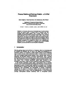
where n is the number of nodes in the graph. A feasible coloring, in which adjacent nodes are assigned different colors, is assured by imposing the constraints xip + xjp ≤ 1 p = 1, ..., K (7) for all adjacent nodes (i,j) in the graph. This problem can be re-cast into the form of UQP by using Transformation 1 on the assignment constraints of (6) and Transformation 2 on the adjacency constraints of (7). No new variables are required. Since the model of (6) and (7) has no explicit objective function, any positive value for the penalty P will do. The following example gives a concrete illustration of the re-formulation process. Consider the graph given in Figure 1 and assume we want find a feasible coloring of the nodes using 3 colors. Our satisfiablity problem is that of finding a solution to: xi1 + xi2 + xi3 = 1 xip + xjp ≤ 1
i = 1, 5 p = 1, 3
(8) (9)
(for all adjacent nodes i and j) In this traditional form, the model has 15 variables and 26 constraints. To recast this problem into the form of UQP, we use Transformation 1 on the
Modeling and Solving Combinatorial Optimization Problems
111
Fig. 1. Example of a graph for the K-Coloring Problem.
equations of (8) and Transformation 2 on the inequalities of (9). Arbitrarily choosing the penalty P to be 4, we get the equivalent problem: ˆ UQP(Pen) : min xQx ˆ matrix is: where the Q
−4 4 4 4 0 0 0 0 0 0 0 0 4 0 0 4 −4 4 0 4 0 0 0 0 0 0 0 0 4 0 4 4 −4 0 0 4 0 0 0 0 0 0 0 0 4 4 0 0 −4 4 4 4 0 0 4 0 0 4 0 0 0 4 0 4 −4 4 0 4 0 0 4 0 0 4 0 0 0 4 4 4 −4 0 0 4 0 0 4 0 0 4 0 0 0 4 0 0 −4 4 4 4 0 0 0 0 0 ˆ = 0 0 0 0 4 0 4 −4 4 0 4 0 0 0 0 Q 0 0 0 0 0 4 4 4 −4 0 0 4 0 0 0 0 0 0 4 0 0 4 0 0 −4 4 4 4 0 0 0 0 0 0 4 0 0 4 0 4 −4 4 0 4 0 0 0 0 0 0 4 0 0 4 4 4 −4 0 0 4 4 0 0 4 0 0 0 0 0 4 0 0 −4 4 4 0 4 0 0 4 0 0 0 0 0 4 0 4 −4 4 0 0 4 0 0 4 0 0 0 0 0 4 4 4 −4
ˆ yields the feasible coloring: Solving this unconstrained model, xQx, x11 , x22 , x33 , x41 , x53 = 1 all other xij = 0 This approach to coloring problems has proven to be very effective for a wide variety of coloring instances from the literature. Later in this paper we present some computational results for several standard K-coloring problems. An extensive presentation of the xQx approach to a variety of coloring problems, including a generalization of the K-coloring problem considered here, is given in Kochenberger, Glover, Alidaee and Rego [KGAR02].
112
Gary A. Kochenberger and Fred Glover
3 Solving UQP Employing the UQP unified framework to solve combinatorial problems requires the availability of a solution method for xQx. The recent literature reports major advances in such methods involving modern metaheuristic methodologies. The reader is referred to references [AHA98, AAK99, Bea99, BS94, BHS89, CS94, GARK02, GKAA99, GKA98, KTN00, Lau70, LAL97, MF99, Pau95, PR90] for a description of some of the more successful methods. The pursuit of further advances in solution methods for xQx remains an active research arena. In the work reported here, we used a basic tabu search method due to Glover, Kochenberger, and Alidaee [GL97, GKAA99, GKA98]. A brief overview of the approach is given below. For complete details the reader is referred to the aforementioned reference. Our TS method for UQP is centered around the use of strategic oscillation, which constitutes one of the primary strategies of tabu search. The method alternates between constructive phases that progressively set variables to 1 (whose steps we call “add moves”) and destructive phases that progressively set variables to 0 (whose steps we call “drops moves”). To control the underlying search process, we use a memory structure that is updated at critical events, identified by conditions that generate a subclass of locally optimal solutions. Solutions corresponding to critical events are called critical solutions. A parameter span is used to indicate the amplitude of oscillation about a critical event. We begin with span equal to 1 and gradually increase it to some limiting value. For each value of span, a series of alternating constructive and destructive phases is executed before progressing to the next value. At the limiting point, span is gradually decreased, allowing again for a series of alternating constructive and destructive phases. When span reaches a value of 1, a complete span cycle has been completed and the next cycle is launched. The search process is typically allowed to run for a pre-set number of span cycles. Information stored at critical events is used to influence the search process by penalizing potentially attractive add moves (during a constructive phase) and inducing drop moves (during a destructive phase) associated with assignments of values to variables in recent critical solutions. Cumulative critical event information is used to introduce a subtle long term bias into the search process by means of additional penalties and inducements similar to those discussed above. Other standard elements of tabu search such as short and long term memory structures are also included.
4 Applications To date several important classes of combinatorial problems have been successfully modeled and solved by employing the unified framework. Our results
Modeling and Solving Combinatorial Optimization Problems
113
with the unified framework applied to these problems have been uniformly attractive in terms of both solution quality and computation times. While our solution method is designed for the completely general form of UQP, without any specialization to take advantage of particular types of problems reformulated in this general representation, our outcomes have typically proved competitive with or even superior to those of specialized methods designed for the specific problem structure at hand. Our broad base of experience with UQP as a modeling and solution framework includes a substantial range of problem classes including: Quadratic Assignment Problems Capital Budgeting Problems Multiple Knapsack Problems Task Allocation Problems (distributed computer systems) Maximum Diversity Problems P-Median Problems Asymmetric Assignment Problems Symmetric Assignment Problems Side Constrained Assignment Problems Quadratic Knapsack Problems Constraint Satisfaction Problems (CSPs) Set Partitioning Problems Fixed Charge Warehouse Location Problems Maximum Clique Problems Maximum Independent Set Problems Maximum Cut Problems Graph Coloring Problems Graph Partitioning Problems Number Partitioning Problems Linear Ordering Problems Number Partitioning Problems. Additional test problems representing a variety of other applications (which do not have “well-known” names) have also been reformulated and solved via UQP. In the section below we report specific computational experience with some of the problem classes listed above Additional applications are discussed by Boris and Hammer [BH91] and Lewis, Alidaee and Kochenberger [LAK04].
5 Illustrative Computational Experience Sections 1 and 2 of this paper presented small examples intended to illustrate the mechanics of the transformation process. Here, we highlight our computational experience with several well-known problem classes. In each case, we specify the standard problem formulation, comment on the transformation(s)
114
Gary A. Kochenberger and Fred Glover
used to recast the problem into the form of UQP, and summarize our computation experience. It is not our objective here to provide a comprehensive comparison with the best known methods for the problem classes considered below. Rather, our purpose in this section is to provide additional validation of the potential merits of this unified approach. Nonetheless, the results shown below are very attractive and motivate such head-to-head comparisons in future studies. 5.1 Warehouse Location: (Single source, Uncapacitated) Zero/One formulation: min
n m P P
i=1 j=1 m P
cij xij +
m P
fi yi
i=1
xij = 1 j = 1, . . . , n
i=1
xij ≤ yi ∀ (i, j) x, y binary
Recast as xQx: • Complement the y variables (to enable the use of transformation # 2) • Use both transformations • No new variables required Computational Experience: • Total number of Problems Solved: 4 # variables 55 210 410 820
m 5 10 10 20
n # TS cycles Soln Time (sec) Soln Optimal? 10 20 < 1 sec Yes 20 50