1
A unified framework for modeling and implementation of hybrid systems with synchronous controllers
arXiv:1501.05936v1 [cs.SY] 23 Jan 2015
Avinash Malik and Partha Roop Abstract—This paper presents a novel approach to including non-instantaneous discrete control transitions in the linear hybrid automaton approach to simulation and verification of hybrid control systems. In this paper we study the control of a continuously evolving analog plant using a controller programmed in a synchronous programming language. We provide extensions to the synchronous subset of the SystemJ programming language for modeling, implementation, and verification of such hybrid systems. We provide a sound rewrite semantics that approximate the evolution of the continuous variables in the discrete domain inspired from the classical supervisory control theory. The resultant discrete time model can be verified using classical model-checking tools. Finally, we show that systems designed using our approach have a higher fidelity than the ones designed using the hybrid automaton approach. Index Terms—Hybrid automata, Synchronous languages, Semantics, Compilers, Verification, Control theory.
F
1
I NTRODUCTION
M
ODERN closed loop control systems consist of a physical process (termed the plant) controlled by a discrete embedded controller. The plant is a continuously evolving (analog) system, which is sampled by an analog to digital converter at specific intervals. These samples are then input into the discrete controller, which makes decisions depending upon the control logic and feeds the resultant outputs back to the plant to control it. The continuous time nature of the plant and the discrete time nature of the controller together form a hybrid system. The Linear Hybrid Automaton [1] is arguably the most popular approach for modeling such hybrid systems. A linear hybrid automaton captures the continuous evolution of the plant model as first order ordinary differential equations (ODEs). In every control mode of the discrete controller, the plant variables evolve according to a set of ODEs, until an invariant condition holds. As soon as the invariant condition is violated, an instantaneous switch is made by the controller to a different control mode. The continuous variables in the plant model can now evolve with a new set of ODEs. Thus, the controller changes the plant behavior through this mode switch. Control systems are reactive systems [2] that have an ongoing interaction with their respective plant in terms of discrete time steps. At the start of each time step, the inputs from the plant are captured, a reaction function is called to process these inputs, and finally the outputs are emitted back to the plant. Synchronous languages such as Esterel [3], Lustre [4], Signal [5] are used extensively to implement such reactive systems, since synchronous programs can be translated into transition systems in • A. Malik and P. Roop are with the Department of Electrical and Computer Engineering, University of Auckland, Auckland, NZ, E-mail:
[email protected],
[email protected]
polynomial time even with exponentially large number of states. Furthermore, model-checking of temporal logic specifications [6] can be directly performed on these resultant symbolic transition systems to guarantee functional and real-time properties of the controller. Synchronous languages, operate based on the principle of synchrony hypothesis, which requires that the reaction function takes zero time and the outputs are produced instantaneously. Given the instantaneous mode switch of the hybrid automaton and the zero delay computation model of the synchronous languages; it should not be surprising then that controllers modeled in hybrid automaton should be implemented with synchronous languages since semantically, the discrete step: mode switch and the reaction function in both models takes zero time. However, in a real system no controller takes zero time. The synchronous language community has addressed this problem by considering the worst case reaction time (WCRT) of a synchronous program [7]. For a synchronous controller; the WCRT, which is akin to the critical path of a program, determines the inter-arrival time of input events. Statically obtaining a tight WCRT for synchronous controllers is a well studied problem [8], [9], [7]. To the best of our knowledge an equivalent approach to incorporating time-delayed mode switches has not been addressed by the hybrid automaton community. Consequently, any results obtained from a system modeled using a hybrid automaton has low fidelity, i.e., does not behave as expected due delays in making control decisions. In this paper our main contribution is: a powerful language with a precise formal semantics that allows the modeling, verification and implementation of non-trivial synchronous controllers with time-delays within their continuous environment. Our contributions can be refined as follows:
2
Automatic, compiler driven, symbolic representation of the hybrid systems designed in the proposed hybrid synchronous language called HySysJ. • A precise formal and novel natural semantics for compilation of hybrid systems. • The discrete approximation of hybrid system designed in HySysJ based on discrete linear time invariant systems from classical supervisory control theory [10]. Rest of the paper is arranged as follows: Section 2 gives a detailed description of the current state of the art in hybrid system design, highlighting the deficiencies. Section 3 introduces the preliminaries required to read the rest of the paper. We motivate the problem using an example in Section 4. The basic language definition is provided in Section 5, which is further extended with continuous time constructs and semantics in Section 6. The relation of the proposed approach to classical supervisory control theory is presented in Section 7. The verification procedure carried out on the motivating example in the resultant new language is given in Section 8. Finally, we conclude in Section 9. •
2
R ELATED
WORK
Many languages have been proposed for modeling and verification of Hybrid systems. A good survey can be found in [11]. The first class of languages are the hardware description languages enhanced with the analog mixed signal (AMS) extensions, such as; VHDL-AMS and SystemC-AMS [12], [13]. These languages lack any sort of formal semantics and hence, cannot be used for formal verification. The second class is the data-flow languages such as Z´elus and SCADE/Lustre [14], [4], which approximate the continuous ODEs. This approach of approximating the continuous ODE behavior is essential, because model-checking most system properties, including safety properties, are known to be undecidable for general hybrid systems [1]. The aforementioned dataflow languages are also endowed with formal mathematical semantics. This conjunction of approximation of continuous behavior along with formal mathematical foundations makes these languages potentially suitable for model-checking. But, unlike us, the overall hybrid model does not account for the non-zero mode-switch times and hence, these programming languages suffer from the same problems as the hybrid automata. Finally, the work closest to the one described in this article is done by: (1) Closse et al. [15], where they extend the Esterel language to model timed automata [16], i.e., ODEs with rate of change always equal to 1. In this proposal we are able to model the more general hybrid rather than its subset timed automaton and (2) Baldamus et al. [17], which is a seminal work in extending synchronous imperative languages to model hybrid automaton. This work is extended further and completed by giving a formal treatment by Bauer et al. [18]. The work described herein differs significantly from both; [18] and [17] in that they do not approximate the continuous
behavior of the plant, instead all discrete transitions are carried out and then a so called continuous phase is launched, which models the continuous evolution of the plant until the invariant condition holds, just like in hybrid automaton. Since these approaches derive their semantics from hybrid automaton, they inherit the same problem described in Section 4, i.e., non-zero modeswitch transitions cannot be captured in the semantics. Overall, the formal foundations of the modeling/implementation language proposed in this paper are truly unique, since the semantics unify the real-time analysis of synchronous programs [7] and the hybrid modeling languages into a single framework inspired from classical supervisory control theory.
3
P RELIMINARIES
In this section we give the background information required for understanding the rest of the paper. 3.1
The hybrid automaton
We use the definition of linear Hybrid automaton from [1]. Definition 1. A hybrid automaton H is a tuple (Loc, V ar, Con, Lab, Edge, Act, Inv, Init) where • (Loc, V ar, Con, Lab, Edge, Act, Inv, Init) is a labelled transition system with Loc a finite set of locations, realvalued variables V ar, V the set of valuation v : V ar → R, and Σ = Loc × V the set of states, Init ⊆ Σ of initial states. V ar • A function Con : Loc → 2 assigning a set of controlled variables to each location • a finite set of labels Lab, including the stutter label τ ∈ Lab. • Act (Activities) is a function assigning a set of activities f : R≥0 → V to each location (l ∈ Loc) which are time-invariant meaning that f ∈ Act(l) implies (f + t) ∈ Act(l) where (f + t)(t0 ) = f (t + t0 ), ∀t0 ∈ R≥0 • a function Inv assigning an invariant Inv(l) ⊆ V to each location l ∈ Loc. V2 • A finite set Edge ⊆ Loc × Lab × 2 × Loc of edges including τ -transitions (l, τ, Id, l) for each location l ∈ Loc with Id = {(v, v 0 )|∀x ∈ Con(l).v 0 (x) = v(x)}, and where all edges with label τ are τ -transitions. Definition 2. The semantics of a hybrid automaton H is given by the operational semantics consisting of two rules, one for discrete instantaneous transition steps and one for continuous time steps. • Discrete step semantics (mode-switch semantics): (l, a, (v, v 0 ), l0 ) ∈ Edge v 0 ∈ Inv(l0 ) a
(l, v) − → (l0 , v 0 ) •
Time step semantics f ∈ Act(l) f (0) = v f (t) = v 0 t ≥ 0 f ([0, t]) ⊆ Inv(l)) t
(l, v) → − (l0 , v 0 )
3
Storage1
Position α
First carousel 0
Second carousel
A/D
D/A
I2 I1
O1
O2
Path1
β
Θ
ϒ
start
Plant
Diverter
S0 I1&&!I2 /O1
Path2
S1
S1
S2 S3
TRDC
Storage2
Fig. 1: The pictorial representation of the manufacturing control system a
t
An execution step →=− →∪→ − of H is either a discrete step or a time step. A path π of H is a sequence σ0 → σ1 . . . with σ0 = (l0 , v0 ) ∈ Init, v0 ∈ Inv(l0 ), and σ0 → σi+1 ∀i ≥ 0. 3.1.1 An example linear hybrid automaton We will use a closed loop manufacturing system example shown in Figure 1 to elaborate the semantics of hybrid automata. Consider that we are designing an automated icecream manufacturing system as shown in Figure 1. The system consists of two carousel belts that carry an icecream to either Storage1 or Storage2 depending upon the RFID tag on the ice-cream. The size of the first carousel is β × γ units. A diverter is placed at the end of the first carousel, β units from the start. A tag reader and diverter controller (TRDC) is placed at position α from the start of the first carousel. When the ice-cream is detected, the TRDC reads the tag on the ice-cream and then sends a control message to the diverter in order to move it into the correct position, so that once the ice-cream reaches position β, it is diverted to the correct storage station. The detection of the ice-cream on the first carousel is indicated by the emission of signal S1. Signal S2, emitted from the TRDC, moves the diverter θ arc-length units in order to divert the ice-cream to Storage1, while signal S3 does the opposite. Furthermore, the carousel and the diverter move at a constant velocity of 1. The hybrid automaton modeling the manufacturing system is shown in Figure 2a. The elements of the tuple defining the syntax of the hybrid automaton are indicated in Figure 2a for sake of understanding. Initially, the ice-cream and the diverter are at position 0, denoted by the continuous variables x and y, respectively. In mode A, the ice-cream travels on the first carousel at a constant velocity of 1 until it reaches position α. As soon as the ice-cream reaches α, signal S1 is emitted with the TAG value Storage1, say. Signal S2 is emitted instantaneously and the hybrid automaton moves to mode B. In this mode, the ice-cream and the diverter, both move at a constant velocity until the diverter covers
1
T/{}
!I1&&I2/ F,O2
S2
2
3
4
5
6
logical ticks
I1 O1
I2 O2 (a) Synchronous controller control-(b) Synchronous controller timling a plant ing diagram
Fig. 3: An example synchronous controller and its timing diagram the distance of θ arc-length units. Finally, a transition is made to mode D, where any further distance until β is covered by the ice-cream and then the ice-cream moves onto the second carousel and is placed into the correct storage. The movement of the ice-cream for this hybrid automaton assuming α = 3, β = 10 and θ = 6 is shown in Figure 2a. Assuming instantaneous discrete modeswitch model of the hybrid automaton, choosing α = 3 is a feasible solution as seen in Figure 2a. The ice-cream is detected at position 3 on the first carousel and an instantaneous move is made to control mode B where the ice-cream moves another 6 units ending up at position 9 when the hybrid automaton is in mode D, which is less than β = 10. 3.2
The synchronous controller
Definition 3. A synchronous controller is a tuple (Q, q0 , I, O, A, T ) where: • Q is the set of states • q0 ∈ Q is the starting state • I is the set of input signals • O is the set of output signals • A is the set of actions A O • T is the transition relation: T ⊆ Q×B(I)×2 ×2 ×Q. B(I) is a Boolean expression over the symbols in I. Simply put, a synchronous controller is a directed graph with edges carrying the labels of the form b/A0 , O0 : b ∈ B(I), A0 ⊆ A, O0 ⊆ O. Intuitively, each edge can be taken if the Boolean condition on the edge holds true. Furthermore, actions (functions) are performed and output signals emitted upon taking the transition. 3.2.1 The timing semantics of synchronous controllers Figure 3a shows a simple example of a synchronous controller controlling a plant. The controller’s input signal set is {I1, I2} and output signals are produced from the set {O1, O2}. The transition system for the controller is also shown in Figure 3a. There are three states in the transition system. The initial state is labeled S0. When signal I1 is produced from the plant, the
4 C
l
ntro
r co ns o
atio Loc
es mod
o St
= S1 1 : α 3 = = S
ge
ra
2
x˙ = 1 y˙ = −1 y≥0 y=0 S3 := 0
∧
A
x := 0 y := 0
x
x˙ = 1 x≤α
x˙ = 1 y˙ = 1 y≤θ
10 9
Movement of ice−cream on first carousel with zero−delay mode−switch 10 OK 9
x = α ∧ S1 = Storage1 S2 := 1 x x =β := 0
Invariants
x (units)
B
Labels
S2 := 0 y=θ D
Activities
3
3
x˙ = 1 x≤β
time (units) 3
(a) The hybrid automaton modelling the manufacturing control system
3 5
5
9 10 9 10
(b) The behavior of the manufacturing control system as modeled by the hybrid automaton
Fig. 2: A simple carousel control system and its hybrid automaton controller makes a transition to state S1. In the process also emitting signal O1 back to the plant. Next, when signal I2 is produced from the plant, the controller makes a transition to state S2. Furthermore, the controller performs an action F and outputs signal O2 back to the plant.
The timing diagram for the controller is shown in Figure 3b. Every synchronous controller, following the zero delay model [3], progresses in lockstep with a logical clock tick. The inputs are captured from the plant at the start of the logical tick, a reaction function is called to process these inputs (in this case the reaction function is the transition system in Figure 3a) and finally the outputs are produced at the end of the tick. The logical ticks are shown as bars in Figure 3b. At logical tick 1, the input signal I1 is captured from the plant, and the output signal O1 is instantaneously produced at the end of the logical tick. Similarly, input signal I2 is captured at the start of tick 4 and output signal is emitted back to the plant at the end this tick – instantaneously.
Unfortunately, execution of every reaction to the input signals takes some δ physical time. The zero delay model implicitly requires that the reaction to the input signals be fast enough in order to not miss any input events from the plant. In order to satisfy this implicit restriction, we need to calculate the Worst Case Reaction Time (WCRT) from amongst all the reaction times, which needs to be shorter than the inter-arrival between any two incoming events. Formally, let {δ1 , . . . , δN } be the set of all possible reaction times for some synchronous controller. Then, ∃i ∈ N , where W CRT = max(δi ). WCRT of any synchronous controller can be calculated statically irrespective of the plant model. Many different techniques exist for the calculation of the WCRT of a synchronous controller [9].
4
T HE
PROBLEM OF TIME - DELAYED MODE SWITCHES
Let us revisit the manufacturing control system example in Section 3.1.1 and use a synchronous language to implement the TRDC controller that performs the discrete mode switches in Figure 2a. Since the length (β), the width (θ) of the first carousel and the speed of movement of the carousel and the diverter are all fixed, we only need to place the TRDC at the correct position on the first carousel so that the diverter is in the correct position by the time ice-cream reaches position β. Our goal is to statically verify that any ice-cream on the first carousel will be diverted to the correct storage depending upon its tag. A hybrid automaton should help us model this system to guarantee this safety property. Note that the reader should interpret the term verify loosely, because the reachability problem for hybrid automata are known undecidable [19]. 4.1 The hybrid automaton and the worst case reaction time of synchronous controllers The movement of the ice-cream in the real system with the TRDC placed at position 3 (as obtained from the hybrid automaton model) is shown in Figure 4a, bottom graph. Every decision made by the controller does take some time. In case of synchronous controllers, this time is the WCRT. Suppose that W CRT = 2 units for the TRDC controller, then the ice-cream is at position 5 when the hybrid automaton moves to mode B. Now, the system modeled by the hybrid automaton and the real implementation are not in-sync. In fact, when the system enters mode D, the invariant x ≤ β does not hold and the transition is immediately made back to mode A. But, the ice-cream is already at position 11 when the system enters mode D, which is past β = 10 and hence, the ice-cream now moves to Storage2 rather than Storage1 as desired, thereby violating the safety property. Overall, the model does not reflect reality and
5 x (units) Movement of ice−cream on first carousel 10 with ideal synchronous controllers OK 9
stmt stmt0 stmt1
x (units) 10 9
3
10 9
Trajectory modeled by the hybrid automaton
Event time (units) x (units)
3
5
9 10
3
3
time (units)
11
ERROR
3
x (units)
3
op
W CRT
Real sampling with a synchronous controller
Sample 3
Movement of ice−cream in the real−system
time (units) 3
5
9 10 11
Sample W CRT time (units)
2 3 42 3 4
::= stmt0 [“||”stmt] ::= stmt1 [“; ”stmt0 ] ::= |“nothing”|“emit” a|“?”a“ = ”expr |“pause”|“abort”“(”[“immediate”]expr“)”stmt |“if ”“(”expr“)”stmt“else”stmt |“suspend”“(”[“immediate”]expr“)”stmt |[“input”|“output”][type]“signal”a [op “ = ”expr] |“loop”stmt|“{”stmt“}” ::= “op+”|“op∗”
Fig. 5: The core kernel statements of the synchronous subset of SystemJ. The terminals appear within double quotes, and angular brackets indicate optional syntactic components.
(a) Difference between the modeled sys-(b) Missed item tag due to WCRTthe discrete transitions in differential equations. But, tem and the real system.
Fig. 4: The different movement of the ice-cream – hybrid automaton model vs. the real system needs to be modified. One might assume that the transition time of the controller is orders of magnitude smaller compared to the speed of movement of the ice-cream on the carousel and hence, can be considered as zero. This is a very rough approximation as indicated in [20]. There are data acquisition delays, sensor delays, communication delays, computation delays in digital controllers, which cannot be ignored with the slight of hand. These delays need to be accounted for in the WCRT of the embedded controller. 4.2 The hybrid automaton, the worst case reaction time and the synchrony hypothesis Every synchronous program can be statically analyzed to find its WCRT. As mentioned before (see Section 3.2) the synchrony hypothesis is guaranteed iff the inter-arrival time of input events is less than or equal to W CRT . For the manufacturing system example W CRT = 2, hence, the synchronous control logic (TRDC), in the worst case, samples inputs every 2 units of time. An input is generated when the ice cream reaches position 3 (since α = 3), but under the synchrony assumption, this input is missed as this input event is not aligned with the edge of the controller clock, i.e., it is not divisible by W CRT = 2 (see Figure 4b). An event driven system would, on the other hand, easily capture this input event. Hence, there is an implicit assumption in the hybrid automaton that the control logic is event driven rather than clock-driven as is the case with synchronous controllers. This is yet another problem that needs to be addressed when designing synchronous controllers. The aforementioned problems occur due to the nonzero reaction time of the synchronous controllers. More precisely, the plant makes progress while the controller carries out internal computations, unlike in the hybrid automaton where these discrete mode-switches zero time. This plant behavior could be modeled by labeling
the hybrid automaton with this solution does not bode well with the semantics of the hybrid automaton. The time for the discrete transition depends upon the implementation of the controller, which differs depending upon the underlying platform, compiler technology, etc. Hence, if we were to simply label the discrete transitions with differential equations, the evolution of the continuous plant variables would depend upon the speed of the controller, which is in stark contrast to the semantics of the hybrid automaton [1]. In light of these problems we need a new programming model for design and verification of hybrid systems. In the rest of the paper we present a power language called HySysJ that: (1) results in high fidelity hybrid system models, by incorporating time-delayed mode switching, (2) allows automatically extracting controllers for implementation from the hybrid model and (3) allows for automatic formal verification of the hybrid system.
5
T HE
BASE LANGUAGE
The proposed language HySysJ builds atop the synchronous subset of the SystemJ [21] programming language, which is itself inspired from Esterel [3]. The core kernel statements of the language are given in Figure 5. The core synchronous language constructs in SystemJ are borrowed directly from Esterel. The nothing construct terminates instantaneously and is primarily used in the structural operational semantics during term rewriting. Every signal is declared via the signal declaration statement. The type declaration for a signal is optional. A non-typed signal is considered to be a pure signal whose status can be set to true for one logical tick by emitting it (via emit) and is f alse if it is not emitted in that logical tick. A valued signal has a value and a status. Every valued signal is uniquely associated with one of the types: ratio, integer, or boolean. A signal can be emitted multiple times with different values in the same logical tick. In such cases, signal values are combined with operators defined during signal declaration. Only associative and commutative operators (e.g., op+ and op∗) are permitted over signal values
6
1
Tick 1
1 2 3 4
signal S, A, B; emit S; if (S) emit A else emit B; pause
signal S, A, B; emit S; pause; //additional pause if (S) emit A else emit B; pause
stmt1 stmt2
S,B
Tick 1
1 2 3 4 5
Fig. 7: Code snippet – incorrect in Esterel, but correct in SystemJ
(b) SystemJ logical timing behavior
(a) Synchronous program code snippet 1
S
stmt3
Tick 2
::= stmt2 ::= |“cont”a [op “ = ” expr] |“cont”a [“ = ” expr] | a = expr |“do“{”stmt3 “}”“until”“(”expr“)” ::= | a“0 ” = expr | a“0 ” = expr[“||”stmt3 ]
(a) The syntactic constructs for continuous variable declaration and manipulation
A
(d) SystemJ logical timing behavior
1 2 3 4 5 6 7
(c) Synchronous program code snippet 2
Fig. 6: SystemJ vs. Esterel logical timing behavior and everything must be well-typed in the expected way. Unlike the status of a signal, the value of a signal is persistent over logical ticks. A block of statements can be preempted or suspended for a single tick using abort and suspend constructs, respectively. The if construct is the usual branching construct, operating on the status or values of signals. Moreover, one or more of the aforementioned statements can be run in lockstep parallel using the synchronous parallel operator ||. Finally, the loop construct is used to write temporal loops, whereby each iteration consumes a logical tick via the pause construct. The synchronous semantics of SystemJ differs from Esterel in one significant way: the emission of every signal is delayed by a single logical tick and is only visible in the next iteration of the synchronous program. We describe these so called delayed signal semantics using simple code snippets shown in Figure 6. Figure 6a shows a very simple synchronous program. Three pure signals S, A, and B are declared. Signal S is emitted and then its status is checked for presence, if this signal has been emitted, then signal A is emitted, else signal B is emitted. Finally, the program ends with the pause statement indicating the end of the logical tick. The logical timing behavior of this SystemJ program is shown in Figure 6b. In SystemJ, the emission of signal makes its visible only in the next logical tick, hence, this program emits signal B in the first logical tick. The logical timing behavior achieved by slightly changing the program (inserting an additional pause construct) is shown in Figures 6c and 6d. In this case, since signal S is emitted in tick-1, its status is true in tick-2 and hence, SystemJ following the so called delayed signal semantics emits signal A in the second tick. Valued signals follow rules similar to signal statuses, i.e., reading a value of the signal (e.g., ?S) always gives the value from the previous logical tick or the default value (0 usually), while setting the value of the signal (e.g., ?S = 2) always sets the current value. The previous
?S = ?S + 1
signal R; abort (R) loop { a = a + ρ * WCRT; if (!TTL ([a0 = ρ], expr, {a})) emit R; pause }
(b) The rewrite for the do {a0 = ρ}until(expr)}. 1 2 3 4 5 6 7
derived
construct:
signal R; abort (R) loop { a = a + ρ * WCRT; b = b + σ * WCRT; if (!TTL ([a0 = ρ, b0 = σ], expr, {a, b})) emit R; pause }
(c) The rewrite for the do {a0 = ρ||b0 = σ}until(expr)}.
derived
construct:
Fig. 8: The continuous variables and derived construct operating on these variables in HySysJ value of the signal is updated to the current value at the end of the logical tick. This so called delayed signal semantics implicitly avoid plethora of problems that plague Esterel programs, related to causality. Consider the code snippet in Figure 7. In case of Esterel, the value of signal S is fed back to itself in the same logical tick, and hence, in Esterel, one needs to check that ?S == (?S + 1), which obviously has no solution. But, in SystemJ, since the signal values are only ever updated at the end of a logical tick, the program in Figure 7 is computable. Now that we have described the base language and its syntactic constructs, we are ready to introduce the continuous elements into the synchronous subset of SystemJ that will result in the new HySysJ hybrid system specification language.
6 IN
H YSYS J – INTRODUCING CONTINUOUS TIME SYNCHRONOUS S YSTEM J
The most fundamental modification to the synchronous language described in Section 5 is the introduction of continuous variables and related actions that manipulate these variables. Following standard practice, we will first introduce the syntactic extensions and then describe the semantics.
7
6.1
Syntax of continuous actions
The syntactic extensions to declare and manipulate the continuous variables are given in Figure 8a. Every continuous variable is declared with the qualifier cont. A default value can be specified during declaration. Uninitialized continuous variables take a default value of 0. Furthermore, a commutative and associative operator (op) can be used to combine the values of the continuous variables, just like in case of valued signals. The type of every continuous variable is a ratio. Two forms of syntactic extensions are allowed for manipulating continuous variables: (1) a direct assignment to the continuous variable or use of continuous variables in expressions, called instantaneous actions and (2) writing first order ODEs inside a do until (expr) block that evolve the continuous variables, called flow actions. We use primed symbols (e.g., a0 = c, where c is some constant) to describe these first order derivatives. One or more such ODEs can be specified inside the do block. The synchronous parallel operator || is used to specify more than one ODE inside the do block. Every ODE inside the do block is evaluated simultaneously until the expr (the so called invariant condition) holds true. The until expr is required to evaluate to a Boolean true or f alse value. 6.2 6.2.1
Semantics of continuous actions Instantaneous actions
Instantaneous actions are so called, because the statement terminates instantaneously without consuming a logical tick. Examples of instantaneous actions are shown in Figure 9. These include; assigning a value to a continuous variable, reading the value of a continuous variable, assigning the value of the continuous variable to a valued signal or another continuous variable, etc. Continuous variables, like signals, follow delayed semantics. Hence, using a continuous variable in an expression (right hand side in case of an assignment statement) always gives the value from the previous logical tick or the default value. A new value is assigned to a continuous variable only at the end of the current logical tick. In Figure 10a, continuous variable a is first declared, with a default value of 0, and then assigned a value of 1. Next, an if else block is used to check the value of a. If the value of a is 1, then signal S1 is emitted else signal S2 is emitted. The same program is presented in Figure 10b, except that a pause statement is inserted after the assignment statement: a = 1. In the first case, due to delayed semantics, when the value of a is read in the if expression, the return value is 0 (the default value) and hence, signal S2 is emitted. On the other hand, in Figure 10b when the program flow reaches the if statement, it is the second logical tick and hence, the value of a is 1 (assigned in the previous logical tick) thus signal S1 is emitted.
1 2 3 4
cont a = 0; //declaring a continuous variable with initial value 0 a = 1; // assigning value 1 to continuous variable a if (a == 1) emit S; //continuous variable used in expression. ?S = a; //value of continuous variable a assigned to a valued signal.
Fig. 9: Instantaneous actions on continuous variables in HySysJ 1 2 3 4 5 6
signal S1, S2; //declaring pure signals cont a; //declaring a with default value 0 a = 1; // assigning value 1 to continuous variable a if (a == 1) emit S1 //continuous variable used in expression. else emit S2; pause
(a) Code snippet 1 1 2 3 4 5 6 7
signal S1, S2; //declaring pure signals cont a; //declaring a with default value 0 a = 1; // assigning value 1 to continuous variable a pause; if (a == 1) emit S1 //continuous variable used in expression. else emit S2; pause
(b) Code snippet 2
Fig. 10: Instantaneous actions on continuous variables in HySysJ with delayed semantics It is important to note that the name instantaneous action does not mean that the value of the continuous variable changes instantaneously. Every continuous variable changes its value only at the end of the tick. The name instantaneous action only implies that the statement itself is instantaneous and does not consume logical ticks1 . 6.2.2 Flow actions The flow actions are programmed using do until blocks and are first order ODEs with a constant rate of change. In the example in Figure 11a, continuous variable a is declared and initialized to a value of 0, which is an instantaneous action. Next, this variable evolves continuously until its value is 2 inside a do until block. In the next example, two variables; a and b evolve together until the invariant condition (until expression) holds. One can also combine multiple such flow actions together in synchronous parallel (Figure 11d). Finally, HySysJ also allows preempting flow actions using the standard preemptive constructs from the base language. 6.2.2.1 Semantics and intuitive explanation for simple flow actions: In this section we describe the rewrite semantics of simple flow actions and give the intuitive explanation for these rewrites. A complete formal treatment is provided in Appendix A. Consider the simple flow action in Figure 11a; variable a evolves linearly with time until it reaches the value 2. The R first order ODE in Figure 11a has the solution: a = 1 × dt = 1 × t + C, where 1 is the rate of change of a and C is the initial value of a. Furthermore, the until expression gives the upper bound on this indefinite 1. Every statement, except for pause in HySysJ is instantaneous
8
1 2
cont a = 0; do {a0 = 1} until (a