A Unified Framework for Protecting Sensitive Association ... - CiteSeerX

A Unified Framework for Protecting Sensitive Association Rules in Business Collaboration∗ Stanley R. M. Oliveira1,2 1 Embrapa Inform´atica Agropecu´aria Av. Andr´e Tosello, 209 13083-970 - Campinas, SP, Brasil [email protected]

Osmar R. Za¨ıane2 2 Department of Computing Science University of Alberta Edmonton, AB, Canada T6G 2E8 [email protected] Abstract

The sharing of association rules has been proven beneficial in business collaboration, but requires privacy safeguards. One may decide to disclose only part of the knowledge and conceal strategic patterns called sensitive rules. These sensitive rules must be protected before sharing since they are paramount for strategic decisions and need to remain private. Some companies prefer to share their data for collaboration, while others prefer to share only the patterns discovered from their data. The challenge here is how to protect the sensitive rules without putting at risk the effectiveness of data mining per se. To address this challenging problem, we propose a unified framework which combines techniques for efficiently hiding sensitive rules: a set of algorithms to protect sensitive knowledge in transactional databases; retrieval facilities to speed up the process of protecting sensitive knowledge; and a set of metrics to evaluate the effectiveness of the proposed algorithms in terms of information loss and to quantify how much private information has been disclosed. Our experiments demonstrate that our framework is effective and achieves significant improvement over the other approaches presented in the literature.

Keywords: Privacy-preserving data mining, knowledge protection, competitive knowledge, sensitive knowledge, sensitive rules, privacy-preserving association rule mining.

1

Introduction

In the business world, companies that once fiercely competed must now form cooperative alliances to provide their customers with a whole product [23]. This is collaboration at its best because of the mutual benefit it brings. Such collaboration may occur between competitors or companies that have ∗

Note to referees: A preliminary version of this work appeared in [18, 20, 21]. The entire paper has been rewritten with additional detail throughout. In particular, we substantially improved the paper both theoretically and empirically to emphasize the practicality and feasibility of our approach. In addition, we compared our algorithms with the similar counterparts in the literature by performing a broad set of experiments using real datasets. Most importantly, this evaluation was carried out to suggest guidance on which algorithms perform best under different conditions. This kind of evaluation has not been explored in any detail in the context of data sanitization.

1

conflict of interests, however as a result, the collaborators are aware that they are provided with an advantage over other competitors. Data mining has been used extensively to support business collaboration. In particular, the discovery of association rules from large databases has proven beneficial for companies. Such rules create assets that collaborating companies can leverage to expand their businesses, improve profitability, reduce costs, and support marketing more effectively [6]. In a collaborative project, one company may decide to disclose only part of the knowledge and conceal strategic patterns which we call sensitive rules. These sensitive rules must be protected before sharing since they are paramount for strategic decisions and need to remain private. Some companies prefer to share their data for collaboration, while others prefer to share only the patterns discovered from their data. Despite its benefits in the business world, association rule mining can also, in the absence of adequate safeguards, open new threats to business collaboration. The concern among privacy advocates is well founded, as bringing data together to support data mining projects makes misuse easier [17]. The challenging problem that we address in this paper is: how can companies transform their data to support business collaboration without losing the benefit of mining? Let us consider a motivating example in which knowledge protection in association rule mining really matters. Suppose we have a server and many clients, with each client having a set of sold items (e.g., books, movies, etc). The clients want the server to gather statistical information about associations among items in order to provide recommendations to customers. However, the clients do not want the server to be able to derive some sensitive association rules. In this context, the clients represent companies and the server hosts a recommendation system for an e-commerce application. In the absence of ratings, which are used in collaborative filtering for automatic recommendation building, association rules can be effectively used to build models for on-line recommendations. When a client sends its frequent itemsets to the server, this client sanitizes some sensitive itemsets according to some specific policies. The sensitive itemsets contain sensitive knowledge that can provide a competitive advantage. The server then gathers statistical information from the sanitized itemsets and recovers from them the actual associations. Is it possible for these companies to benefit from such collaboration by sharing association rules while preserving some sensitive rules? The simplistic solution to address the motivating example is to implement a filter after the mining phase to weed out/hide the sensitive discovered rules. However, we claim that trimming some rules out does not ensure full protection. The solution to remove a set of sensitive rules must not leave a trace that could be exploited by an adversary. We must guarantee that some inference channels have been blocked as well. To address this challenging problem, we propose a unified framework for protecting sensitive association rules before sharing. This framework combines techniques for efficiently hiding sensitive patterns: a set of algorithms to protect sensitive knowledge; retrieval facilities to speed up the process of protecting sensitive knowledge; and a set of metrics to evaluate the effectiveness of the proposed algorithms in terms of information loss and to quantify how much private information has been disclosed.

2

Our algorithms require only two scans regardless of the database’s size and the number of sensitive rules that must be protected. The first scan is required to build an index for speeding up the sanitization process, while the second scan is used to remove the sensitive rules from the released database. The previous methods in the literature require as many scans as there are rules to hide [10, 26, 29]. This paper is organized as follows. In Section 2, we provide the basic concepts that are necessary to understand the issues addressed in this paper. In Section 3, we describe the research problem employed in our study. The framework to protect sensitive knowledge in transactional databases is presented in Section 4. We present our heuristics to protect sensitive rules in association rule mining in Section 5. In Section 6, we introduce our sanitizing algorithms which are categorized into two groups: data sharing-based and pattern sharing-based algorithms. The existing solutions in the literature to protect sensitive knowledge are reviewed in Section 7. The experimental results are presented in Section 8. Finally, Section 9 presents our conclusions.

2

Background

In this section, we briefly review the basics of association rules and provide the definitions of sensitive rules and sensitive transactions. Subsequently, we describe the process of protecting sensitive knowledge in transactional databases.

2.1

The Basics of Association Rules

One of the most studied problems in data mining is the process of discovering association rules from large databases. Most of the existing algorithms for association rules rely on the support-confidence framework introduced in [2, 3]. Formally, association rules are defined as follows: Let I = {i1 ,...,in } be a set of literals, called items. Let D be a database of transactions, where each transaction t is an itemset such that t ⊆ I. A unique identifier, called TID, is associated with each transaction. A transaction t supports X, a set of items in I, if X ⊂ t. An association rule is an implication of the form X ⇒ Y , where X ⊂ I, Y ⊂ I and X ∩ Y = ∅. Thus, we say that a rule X ⇒ Y holds in the database D with confidence ϕ if

|X∪Y | |X|

≥ ϕ,

where |A| is the number of occurrences of the set of items A in the set of transactions D. Similarly, we say that a rule X ⇒ Y holds in the database D with support σ if

|X∪Y | N

≥ σ, where N is the number

of transactions in D. While the support is a measure of the frequency of a rule, the confidence is a measure of the strength of the relation between sets of items. A survey of algorithms for association rules can be found in [14].

2.2

Sensitive Rules and Sensitive Transactions

Protecting sensitive knowledge in transactional databases is the task of hiding a group of association rules which contains sensitive knowledge. We refer to these rules as sensitive association rules and define them as follows:

3

Definition 1 (Sensitive Association Rules) Let D be a transactional database, R be a set of all association rules that can be mined from D based on a minimum support σ, and RulesH be a set of decision support rules that need to be hidden according to some security policies. A set of association rules, denoted by SR , is said to be sensitive iff SR ⊂ R and SR would derive the set RulesH . ~SR is the set of non-sensitive association rules such that ~SR ∪ SR = R. A group of sensitive association rules is mined from a database D based on a special group of transactions. We refer to these transactions as sensitive transactions and define them as follows: Definition 2 (Sensitive Transactions) Let T be a set of all transactions in a transactional database D and SR be a set of sensitive association rules mined from D. A set of transactions is said to be sensitive, denoted ST , if ST ⊂ T and ∀ t ∈ ST , ∃ sr ∈ SR such that items(sr) ⊆ t.

2.3

The Process of Protecting Sensitive Knowledge

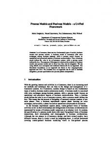
The process of protecting sensitive knowledge in transactional databases is composed of two major steps: identifier suppression and sanitization, as can be seen in Figure 1.

Original Database

Identifier Suppression Step 1

Transactional Database

Sanitization Step 2

Sanitized Database

Figure 1: Major steps of the process of protecting sensitive knowledge. Step 1: Identifier Suppression The first step of the sanitization process refers to the suppression of identifiers (e.g., IDs, names, etc) from the data to be shared. The procedure of removing identifiers allows database owners to disclose purchasing behavior of customers without disclosing their identities [16]. To accomplish that, database owners must transform the data into forms appropriate for mining. After removing identifiers, the selected data which are subjected to mining, can be stored in a single table, also called a transactional database. A transactional database does not contain personal information, but only costumers’ buying activities. Although the deletion of identifiers from the data is useful to protect personal information, we do not argue that this procedure ensures full privacy at all. In many cases, it is very difficult to extract the specific identity of one or more costumers from a transactional database, even combining the transactions with other data. However, a specific transaction may contain some items that can be linked with other datasets to re-identify an individual or and entity [25, 27]. Once the data is transformed into a transactional database, the process of hiding sensitive rules from this transactional database is the next step to be pursued. Step 2: Sanitization

4

After removing the identifiers from the data, the goal now is to efficiently hide sensitive knowledge represented by sensitive rules. In most cases, the notion of sensitive knowledge may not be known in advance. That is why the process of identifying sensitive knowledge requires human evaluation of the intermediate results before the sharing of data for mining. In this context, sensitive knowledge is represented by a special group of rules referred to as sensitive association rules. An efficient way to hide sensitive rules is by transforming a transactional database into a new one that conceals the sensitive rules while preserving most of the non-sensitive ones. The released database is called a sanitized database. To accomplish that, the sanitization process acts on the data modifying some transactions. In some cases, a number of items are deleted from a group of transactions (sensitive transactions) with the purpose of hiding the sensitive rules derived from those transactions. In doing so, the support of such sensitive rules are decreased below a certain disclosure threshold denoted by ψ. Another way to hide sensitive rules is to add new items to some transactions to alter (decrease) the confidence of sensitive rules. For instance, in a rule X → Y , if the items are added to the antecedent part X of this rule in transactions that support X and not Y , then the confidence of such a rule is decreased. Clearly, the sanitization process slightly modifies some data, but this is perfectly acceptable in some real applications [4, 10, 26]. Although the sanitization process is performed to hide sensitive rules only, the side effect of this process also hides some non-sensitive ones. By deleting some items in a group of transactions, the support or even the confidence of non-sensitive rules are also decreased. Therefore, sanitizing algorithms must focus on hiding sensitive rules and, at the same time, reducing the side effect on the non-sensitive rules as much as possible.

3

Knowledge Protection: Problem Definition

In the context of privacy-preserving association rule mining, we do not address privacy of individuals. Rather, we address the problem of protecting sensitive knowledge mined from databases. The sensitive knowledge is represented by a special group of association rules called sensitive association rules. These rules are paramount for strategic decision and must remain private (i.e., the rules are private to the company or organization owning the data). The problem of protecting sensitive knowledge in transactional databases, draws the following assumptions: • Data owners have to know in advance some knowledge (rules) that they want to protect. Such rules are fundamental in decision making, so they must not be discovered. • The individual data values (e.g., a specific item) are not restricted. Rather, some aggregates and relationships must be protected. This approach works in the opposite way to the idea behind statistical databases [1] which prevents against discovering individual tuples. The problem of protecting sensitive knowledge in association rule mining can be stated as follows: If D is the source database of transactions and R is a set of relevant association rules that could be 5

mined from D, the goal is to transform D into a database D0 so that the most association rules in R can still be mined from D0 while others, representing sensitive knowledge, are hidden. In this case, D0 becomes the released database.

4

The Framework for Knowledge Protection

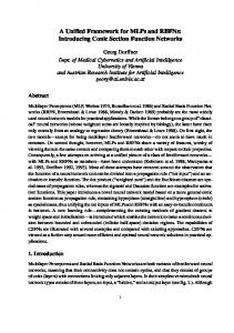
In this section, we introduce the framework to protect sensitive knowledge in association rule mining. As depicted in Figure 2, the framework encompasses an inverted file to speed up the sanitization process, a library of sanitizing algorithms used for hiding sensitive association rules from the database, and a set of metrics to quantify not only how much private information is disclosed, but also the impact of the sanitizing algorithms on the transformed database and on valid mining results. Inverted File

Sensitive Rules

Sanitizing Algorithms

Transaction IDs

Transactional Database

Sanitized Database

Metrics

Figure 2: The framework to protect sensitive knowledge in association rule mining.

4.1

The Inverted File

Sanitizing a transactional database consists of identifying the sensitive transactions and adjusting them. To speed up this process, we scan a transactional database only once and, at the same time, we build our retrieval facility (inverted file) [5]. The inverted file’s vocabulary is composed of all the sensitive rules to be hidden, and for each sensitive rule there is a corresponding list of transaction IDs in which the rule is present. Figure 3(b) shows an example of an inverted file corresponding to the transactional database shown in Figure 3(a). For this example, we assume that the sensitive rules are A,B → D and A,C → D. Note that once the inverted file is built, a data owner will sanitize only the sensitive transactions whose IDs are stored in the inverted file. Knowing the sensitive transactions prevents a data owner from performing multiple scans in the transactional database. Consequently, the CPU time for the sanitization process is optimized. Apart from optimizing the CPU time, the inverted file provides other advantages, as follows:

6

TID

Inverted File

Items

T1 T2 T3 T4 T5 T6

A A A A A B

B B B C B D

C D C D D C

A, B −> D

T1, T3

A, C −> D

T1, T4

Sensitive Rules

(A)

Transaction IDs

(B)

Figure 3: (a) A sample transactional database.

(b) The corresponding inverted file.

• The information kept in main memory is greatly reduced since only the sensitive rules are stored in memory. The occurrences (transaction IDs) can be stored on disk when not fitted in main memory. • Our algorithms require at most two scans regardless of the number of sensitive rules to be hidden: one scan to build the inverted file, and the other to sanitize the sensitive transactions. The previous methods in the literature require as many scans as there are rules to hide [10, 26].

4.2

The Library of Sanitizing Algorithms

In our framework, the sanitizing algorithms modify some transactions to hide sensitive rules based on a disclosure threshold ψ controlled by the database owner. This threshold indirectly controls the balance between knowledge disclosure and knowledge protection by controlling the proportion of transactions to be sanitized. For instance, if ψ = 50% then half of the sensitive transactions will be sanitized, when ψ = 0% all the sensitive transaction will be sanitized, and when ψ = 100% no sensitive transaction will be sanitized. In other words, ψ represents the ratio of sensitive transactions that should be left untouched. The advantage of this threshold is that it enables a compromise between hiding association rules while missing non-sensitive ones, and finding all non-sensitive association rules but uncovering sensitive ones. As can be seen in Figure 2, the sanitizing algorithms are applied to the original database to produce the sanitized one. We classify our algorithms into two major groups: data sharing-based algorithms and pattern sharing-based algorithms, as can be seen in Figure 4. Sanitizing Algorithms Item Grouping Algorithm (IGA) Data Sharing−Based Algorithms Sliding Window Algorithm (SWA) Pattern Sharing−Based Algorithms

Downright Sanitizing Algorithm (DSA)

Figure 4: A taxonomy of sanitizing algorithms. In the former, the sanitization process acts on the data to remove or hide the group of sensitive 7

R’ R

SR

~S R

2 Misses Cost

1

3

Hiding Failure

Artifactual Patterns

Figure 5: Data sharing-based sanitization problems. association rules representing the sensitive knowledge. To accomplish this, a small number of transactions that participate in the generation of the sensitive rules have to be modified by deleting one or more items from them. In doing so, the algorithms hide sensitive rules by reducing either their support or confidence below a privacy threshold (disclosure threshold). In the latter, the sanitizing algorithm acts on the rules mined from a database, instead of the data itself. The algorithm removes all sensitive rules before the sharing process. In Section 6, we introduce our sanitizing algorithms.

4.3

The Set of Metrics

In this section, we introduce the set of metrics to quantify not only how much sensitive knowledge has been disclosed, but also to measure the effectiveness of the proposed algorithms in terms of information loss and in terms of non-sensitive rules removed as a side effect of the transformation process. We classify these metrics into two major groups: Data sharing-based metrics and Pattern sharing-based metrics. a) Data sharing-based metrics are related to the problems illustrated in Figure 5. This figure shows the relationship between the set R of all association rules in the database D, the sensitive rules SR , the non-sensitive association rules ∼SR , as well as the set R0 of rules discovered from the sanitized database D0 . The circles with the numbers 1, 2, and 3 are potential problems that respectively represent the sensitive association rules that were failed to be hidden, the legitimate rules accidentally missed, and the artificial association rules created by the sanitization process. Problem 1 occurs when some sensitive association rules are discovered in the sanitized database. We call this problem Hiding Failure (HF), and it is measured in terms of the percentage of sensitive association rules that are discovered from D0 . Ideally, the hiding failure should be 0%. The hiding failure is measured as follows: HF =

# SR (D0 ) # SR (D)

where # SR (X) denotes the number of sensitive association rules discovered from the database X. 8

(1)

Problem 2 occurs when some legitimate association rules are hidden as a side effect of the sanitization process. This happens when some non-sensitive association rules lose support in the database due to the sanitization process. We call this problem Misses Cost (MC), and it is measured in terms of the percentage of legitimate association rules that are not discovered from D0 . In the best case, this should also be 0%. The misses cost is calculated as follows: MC =

# ∼SR (D) − # ∼SR (D0 ) # ∼SR (D)

(2)

where # ∼SR (X) denotes the number of non-sensitive association rules discovered from the database X. Notice that there is a compromise between the misses cost and the hiding failure. The more sensitive rules we hide, the more non-sensitive rules we miss. This is basically the justification for our disclosure threshold ψ, which with tuning, allows us to find the balance between privacy and disclosure of information whenever the application permits it. Problem 3 occurs when some artificial association rules are generated from D0 as a product of the sanitization process. We call this problem Artifactual Patterns (AP), and it is measured in terms of the percentage of the discovered association rules that are artifacts, i.e., rules that are not present in the original database. Artifacts are generated when new items are added to some transactions to alter (decrease) the confidence of sensitive rules. For instance, in a rule X → Y , if the items are added to the antecedent part X of this rule in transactions that support X and not Y , then the confidence of such a rule is decreased. Artifactual patterns are measured as follows: AP =

|R0 | − |R ∩ R0 | |R0 |

(3)

where |X| denotes the cardinality of X. We could measure the dissimilarity between the original and sanitized databases by computing the difference between their sizes in bytes. However, we believe that this dissimilarity should be measured by comparing their contents instead of their sizes. Comparing their contents is more intuitive and gauges more accurately the modifications made to the transactions in the database. To measure the dissimilarity between the original and the sanitized datasets, we could simply compare the difference in their histograms. In this case, the horizontal axis of a histogram contains all items in the dataset, while the vertical axis corresponds to their frequencies. The sum of the frequencies of all items gives the total of the histogram. So the dissimilarity between D and D’ is given by: n

X 1 [fD (i) − fD0 (i)] × i=1 fD (i)

Dif (D, D0 ) = Pn

(4)

i=1

where fX (i) represents the frequency of the i-th item in the dataset X, and n is the number of distinct items in the original dataset. b) Pattern sharing-based metrics: are related to the problems illustrated in Figure 6. Problem 1 9

conveys the non-sensitive rules (∼SR ) that are removed as a side effect of the sanitization process (RSE ). We refer to this problem as side effect. It is related to the misses cost problem in data sanitization (Data sharing-based metrics). Problem 2 occurs when using some non-sensitive rules, an adversary may recover some sensitive ones by inference channels. We refer to such a problem as recovery factor. Rules to be shared (R’)

Problem 1: Side effect (RSE)

Non−Sensitive Rules ~S R

Sensitive Rules S R

Rules to hide

Rules hidden

Problem 2: Inference

Figure 6: Pattern sharing-based sanitization problems. Side Effect Factor (SEF) measures the number of non-sensitive association rules that are removed as a side effect of the sanitization process. The measure is calculated as follows: SEF =

(|R| − (|R0 | + |SR |)) (|R| − |SR |)

(5)

where R, R0 , and SR represent the set of rules mined from a database, the set of sanitized rules, and the set of sensitive rules, respectively, and |S| is the size of the set S. Recovery Factor (RF) expresses the possibility of an adversary recovering a sensitive rule based on non-sensitive ones. The recovery factor of one pattern takes into account the existence of its subsets. The rationale behind the idea is that all nonempty subsets of a frequent itemset must be frequent. Thus, if we recover all subsets of a sensitive itemset (rule), we say that the recovery factor for such an itemset is possible, and thus we assign it the value 1. However, the recovery factor is never certain, i.e., an adversary may not learn an itemset even with its subsets. On the other hand, when not all subsets of an itemset are present, the recovery of the itemset is improbable, thus we assign value 0 to the recovery factor. In the pattern sharing-based approach, the set of sanitized rules to be shared (R0 ) is defined as R0 = R − (SR + RSE ), where R is the set of all rules mined from a database, SR is the set of sensitive rules, and RSE is the set of rules removed as a side effect of the sanitization process.

5

Heuristics for Protecting Sensitive Rules

The optimal sanitization has been proved to be an NP-hard problem [4]. To alleviate the complexity of the optimal sanitization, we could use some heuristics. An heuristic does not guarantee the optimal solution, but usually finds a solution close to the best one in a faster response time [9].

10

In this section, we describe three heuristics to hide sensitive rules in transactional databases. The first two heuristics act on the data to protect or hide a group of sensitive association rules. After sanitizing a database, the released database is shared for association rule mining. We refer to these heuristics as data sharing-based heuristics. The third heuristic falls into another category that we call pattern sharing-based heuristics. In this approach, the sanitization process acts on the rules mined from a database instead of the data itself. Rather than sharing the data, data owners may prefer to mine their own data and share some discovered patterns. In this case, the sanitization removes not only all sensitive rules but also blocks other rules that could be used to infer the sensitive hidden ones.

5.1

Heuristic 1: Sanitization Based on the Degree of Sensitive Transactions

Our first heuristic for data sanitization is based on the fact that, in many cases, a sensitive transaction (see Section 2.2) participates in the generation of one or more sensitive association rule to be hidden. We refer to the number of sensitive rules supported by a sensitive transaction as the degree of a sensitive transaction, defined as: Definition 3 (Degree of a Sensitive Transaction) Let D be a transactional database and ST a set of all sensitive transactions in D. The degree of a sensitive transaction t, denoted by degree(t), such that t ∈ ST , is defined as the number of sensitive association rules that can be found in t. Our Heuristic 1 has essentially four major steps, as follows: • Step 1: Scan a database and identify the sensitive transactions for each sensitive association rule. This step is accomplished when the inverted file is built; • Step 2: Based on the disclosure threshold ψ, calculate for each sensitive association rule the number of sensitive transactions that should be sanitized and mark them. Most importantly, the sensitive transactions are selected based on their degree (descending order); • Step 3: For each sensitive association rule, identify a candidate item that should be eliminated from the sensitive transactions. This candidate item is called the victim item; • Step 4: Scan the database again, identify the sensitive transactions marked to be sanitized and remove the victim items from them. To illustrate how our presented heuristic works, let us consider the sample transactional database in Figure 7(a). Suppose that we have a set of sensitive association rules SR = {A,B→D; A,C→D}. This example yields the following results: • Step 1: We first scan the database to identify the sensitive transactions. For this example, the sensitive transactions ST containing the sensitive association rules are {T1, T3, T4}. The degrees of the transactions T1, T3 and T4 are 2, 1 and 1 respectively. In particular, the rule A,B→D can be mined from the transactions T1 and T3 and the rule A,C→D can be mined from T1 and T4. 11

• Step 2: Suppose that we set the disclosure threshold ψ to 50%. We then sort the sensitive transactions in descending order of degree. Subsequently, we sanitize half of the sensitive transactions for each sensitive rule. In this case, only the transaction T1 will be sanitized. • Step 3: In this step, the victim items are selected. To do so, we group sensitive rules that share a common item. Both rules share the items A and D. In this case, only one item is selected, say the item D. By removing the item D from T1 the sensitive rules will be hidden from T1 in one step and the disclosure threshold will be satisfied. • Step 4: We perform the sanitization taking into account the victim items selected in the previous step. The sanitized database can be seen in Figure 7(b).

TID T1 T2 T3 T4 T5 T6

Items A A A A A B

B B B C B D

TID

C D C D D C

T1 T2 T3 T4 T5 T6

(a)

Items A A A A A B

B B B C B D

C C D D C

(b)

Figure 7: (a) A copy of the sample transactional database in Figure 3(a); (b) The sanitized database using Heuristic 1. An important observation here is that any association rule that contains a sensitive association rule is also sensitive. Hence, if A,B→D is a sensitive association rule, any association rule derived from the itemset ABCD will also be sensitive since it contains ABD. This is because if ABCD is discovered to be a frequent itemset, it is straightforward to conclude that ABD is also frequent, which should not be disclosed. In other words, any superset containing ABD should not be allowed to be frequent.

5.2

Heuristic 2: Sanitization Based on the Size of Sensitive Transactions

We now introduce the second heuristic to hide sensitive knowledge in transactional databases. The idea behind this heuristic is to sanitize the sensitive transactions with the shortest sizes. The rationale is that by removing items from shortest transactions we would minimize the impact on the sanitized database since the shortest transactions have fewer combinations of association rules. As a consequence, we would reduce the side effect of the sanitization process on non-sensitive rules. Our Heuristic 2 approach has essentially four steps as follows: Step 1: Distinguishing the sensitive transactions from the non-sensitives ones. For each transaction read from a database D, we identify whether this transaction is involved in the generation of any sensitive association rule. If not, the transaction is copied directly to the sanitized database D0 . Otherwise, this transaction is sensitive and must be sanitized. 12

Step 2: Selecting the victim item. In this step, we first compute the frequencies of all items in the sensitive association rules presented in the current sensitive transaction. The item with the highest frequency is the victim item since it is shared by a group of sensitive rules. If a sensitive rule shares no item with the other sensitive ones, the frequencies of its items are the same (freq = 1). In this case, the victim item for this particular sensitive rule is selected randomly. The rationale behind this selection is that removing different items from the sensitive transactions would slightly minimize the support of the legitimate association rules that would be available for being mined in the sanitized database D0 . Step 3: Computing the number of sensitive transactions to be sanitized. Given the disclosure threshold, ψ, set by the database owner, we compute the number of transactions to be sanitized. Every sensitive rule will have a list of sensitive transaction IDs associated with it. In this step, we sort the sensitive transactions computed previously for each sensitive rule. The sensitive transactions are sorted in ascending order of size. Thus, we start sanitizing the shortest transactions. Step 4: Sanitizing a sensitive transaction. Given that the victim items for all sensitive association rules were selected in step 2, they can now be removed from the sensitive transactions. Every sensitive rule now has a list of sensitive transaction IDs with their respective selected victim item. Every time we remove a victim item from a sensitive transaction, we perform a look ahead procedure to verify whether that transaction has been selected as a sensitive transaction for other sensitive rules. If so, and the victim item we just removed from the current transaction is also part of this other sensitive rule, we remove that transaction from the list of transaction IDs marked in the other rules. In doing so, the transaction will be sanitized and then copied to the sanitized database D0 . This look-ahead procedure is done only when the disclosure threshold is 0%. This is because the look-ahead improves the misses cost but could significantly degrade the hiding failure. When ψ = 0, there is no hiding failure (i.e., all sensitive rules are hidden) and thus there is no degradation possible but an improvement in the misses cost. To illustrate how our Heuristic 2 works, let us consider the sample transactional database in Figure 8(a). Suppose that we have a set of sensitive association rules SR = {A,B→D; A,C→D} and we set the disclosure threshold ψ = 50%. This example yields the following results: Step 1: The sensitive transactions are identified. In this case, the sensitive transactions of A,B→D and A,C→D are {T1, T3} and {T1, T4} respectively. Step 2: After identifying the sensitive transactions, we select the victim items. For example, the victim item in the transaction T1 could be either A or D since these items are shared by the sensitive rules and consequently their frequencies are equal to 2. However, the victim item for the sensitive rule A,B→D in T3 is selected randomly because the items A, B, and D have frequencies equal to 1. Let us assume that the victim item selected is B. Similarly, the victim item for the sensitive rule A,C→D, in transaction T4, is selected randomly, say, the item A.

13

Step 3: In this step, we compute the number of sensitive transactions to be sanitize, for each sensitive rule. This computation is based on the disclosure threshold ψ. We selected ψ = 50% for both rules. However, we could set a particular disclosure threshold for each sensitive rule. We also sorted the sensitive transactions in ascending order of size before performing the sanitization in the next step. Step 4: We then sanitize the transactions for each sensitive rule. Half of the transactions for each sensitive rule will be intact since the disclosure threshold ψ = 50%. We start by sanitizing the shortest transactions (sorted in the previous step). Thus, transactions T3 and T4 are sanitized. The released database is depicted in Figure 8(b). Note that the sensitive rules are present in the sanitized database, but with lower support. This is an example of partial sanitization. The database owner could also set the disclosure threshold ψ = 0%. In this case, we have a full sanitization since the sensitive rules will no longer be discovered. In this example, we assume that the victim item in transaction T1 is D since this item is shared by both sensitive rules. Figure 8(c) shows the database after a full sanitization. As we can see, the database owner can tune the disclosure threshold to find a balance between protecting sensitive association rules by data sanitization and providing information for mining. TID T1 T2 T3 T4 T5 T6

Items A A A A A B

B B B C B D

C D C D D C

TID T1 T2 T3 T4 T5 T6

(A)

Items A A A C A B

B C D B C D D B C D

(B)

TID T1 T2 T3 T4 T5 T6

Items A A A C A B

B C B C D D B C D

(C)

Figure 8: (a): A copy of the sample transactional database in Figure 3(a); (b): An example of partial sanitization; (c): An example of full sanitization.

5.3

Heuristic 3: Rule Sanitization With Blocked Inference Channels

Recall that our previous heuristics are classified as data sharing-based heuristics which rely on sanitizing a database before data sharing. Our third heuristic sanitizes sensitive rules from a set of rules mined from a database, while blocking some inference channels. The remaining association rules are shared. This approach falls into the pattern sharing-based heuristics. Before introducing our new heuristic, we briefly review some terminology from graph theory. In particular, we represent the itemsets in a database as a directed graph. We refer to such a graph as a frequent itemset graph and define it as follows: Definition 4 (Frequent Itemset Graph) A frequent itemset graph, denoted by G = (C, E), is a directed graph which consists of a nonempty set of frequent itemsets C, a set of edges E that are 14

TID

List of Items

T1

A

B

C

T2

A

B

C

T3

A

C

D

T4

A

B

C

T5

A

B

A

B

C

D

Level 0

D AB

AC

AD

ABC

(a)

Figure 9: (a) A transactional database.

BC

CD

ACD

Level 1

Level 2

(b)

(b) The corresponding frequent itemset graph.

ordered pairings of the elements of C, such that ∀u, v ∈ C there is an edge from u to v if u ∩ v = u and |v| − |u| = 1, where |x| is the size of itemset x. Figure 9(b) shows a frequent itemset graph for the sample transactional database depicted in Figure 9(a). In this example, the minimum support threshold σ is set to 2. As can be seen in Figure 9(b), in a frequent itemset graph G, there is an order for each itemset. We refer to such an ordering as the itemset level and define it as follows: Definition 5 (The Itemset Level) Let G = (C, E) be a frequent itemset graph. The level of an itemset u, such that u ∈ C, is the length of the path connecting an 1-itemset to u. Based on Definition 5, we define the level of a frequent itemset graph G as follows: Definition 6 (Frequent Itemset Graph Level) Let G = (C, E) be a frequent itemset graph. The level of G is the length of the maximum path connecting an 1-itemset u to any other itemset v, such that u, v ∈ C, and u ⊂ v. In general, the discovery of itemsets in G is the result of top-down traversal of G constrained by a minimum support threshold σ. The discovery process employs an iterative approach in which k-itemsets are used to explore (k + 1)-itemsets. Our Heuristic 3 has essentially three steps, as follows. These steps are applied after the mining phase, i.e., we assume that the frequent itemset graph G is built. The set of all itemsets that can be mined from G, based on a minimum support threshold σ, is denoted by C. Step1: Identifying the sensitive itemsets. For each sensitive rule sri ∈ SR , convert it into a sensitive itemset ci ∈ C. Step2: Selecting subsets to sanitize. In this step, for each itemset ci to be sanitized, we compute its item pairs from level 1 in G, subsets of ci . If none of them is marked, we randomly select one of them and mark it to be removed. Step3: Sanitizing the set of supersets of marked pairs in level 1. The sanitization of sensitive itemsets is simply the removal of the set of supersets of all itemsets in level 1 of G that are marked 15

A

AB

B

AC

C

BC

D Level 0

AD

ABC

ACD

A

CD Level 1

AB

Level 2

B

AC

C

BC

AD

ABC

(a)

D Level 0

ACD

CD Level 1

Level 2

(b)

Figure 10: (a) An example of forward-inference.

(b) An example of backward-inference.

for removal. This process blocks possibilities of inferring sensitive rules. We refer to these possibilities as inference channels that we describe in the next section. In the pattern sharing-based heuristics, an inference channel occurs when someone mines a sanitized set of rules and, based on non-sensitive rules, deduces one or more sensitive rules that are not supposed to be discovered. We have identified some inferences against sanitized rules, as follows: Forward-Inference Channel: Let us consider the frequent itemset graph in Figure 10(a). Suppose we want to sanitize the sensitive rules derived from the itemset ABC. The na¨ıve approach is simply to remove the itemset ABC. However, if AB, AC, and BC are frequent, a miner could deduce that ABC is frequent. A database owner must assume that an adversary can use any inference channel to learn something more than just the permitted association rules. We refer to this inference as a forward-inference channel. To handle this inference channel, we must also remove at least one subset of ABC (randomly) in level 1 of the frequent itemset graph. This complementary sanitization is necessary. In the case of a deeper graph, the removal is done recursively up to level 1. Thus, the items in level 0 of the frequent itemset graph are not shared with a second party. We could also remove subsets of ABC recursively up to level 0. In this case, the balance between knowledge protection and knowledge discovery should be considered in the released set of rules, since more frequent patterns are lost by the sanitization process. Backward-Inference Channel: Another type of inference occurs when we sanitize a non-terminal itemset. Based on Figure 10(b), suppose we want to sanitize any rule derived from the itemset AC. If we simply remove AC, it is straightforward to infer the rules mined from AC, since both ABC and ACD are frequent. We refer to this inference as a backward-inference channel. To block this inference channel, we must remove any superset that contains AC. In this particular case, ABC and ACD must be removed as well. This kind of inference clearly shows that rule sanitization is not a simple filter after the mining phase to weed out or hide the sensitive rules. Trimming some rules out does not ensure full protection. Some inference channels must be blocked as well. To illustrate how our Heuristic 3 works, let us consider the frequent itemset graph depicted in Figure 9(b). This frequent itemset graph corresponds to the sample transactional database in Figure 9(a), 16

A

B

AB*

AC

ABC* Step 2

C

BC

AD

D Level 0

CD

ACD

Step 1

A

Level 1

B

AC

Level 2

C

BC

AD

D Level 0

CD

ACD

Level 1

Level 2

Step 3

Frequent itemset graph before sanitization

Frequent itemset graph after sanitization

Figure 11: An example of a frequent itemset graphs before and after sanitization. with minimum support threshold σ = 2. Now suppose that we are sanitizing the sensitive rule A,B→C before sharing the frequent itemset graph. This example yields the following results: Step 1: Each sensitive rule is converted into its corresponding frequent itemset. In this case, the rule A,B→C is converted into the itemset ABC. Step 2: In this step, the subsets for each rule are selected. In general, the subsets are selected from the level 1 in the frequent itemset graph. For this example, considering that there is no subset marked, we select one of the subsets of ABC randomly. If we had subsets marked previously, we would select one already marked to optimize the sanitization process. Let us assume that we selected the subset AB randomly. Then the subset AB was added to the list that contains all the marked pairs to be sanitized. Step 3: In this step, the sanitization takes place. We remove all supersets of each pair marked to be sanitized. In this case, all the supersets of AB will be removed. Figure 11 shows the frequent itemset graphs before and after the rule sanitization. The sanitized frequent itemset graph is shared for association rule mining.

6

The Sanitizing Algorithms

In this section, we introduce our sanitizing algorithms to protect sensitive knowledge in transactional databases. These algorithms correspond to the heuristics presented in Section 5 and are categorized into two groups: data sharing-based and pattern sharing-based algorithms.

6.1

The Item Grouping Algorithm

The Item Grouping Algorithm, denoted by IGA, relies on Heuristic 1. The main idea behind this algorithm is to group sensitive rules in groups of rules sharing the same itemsets. If two sensitive rules intersect, by sanitizing the sensitive transactions containing both sensitive rules, one would take care of hiding these two sensitive rules at once and consequently reduce the impact on the released database. However, clustering the sensitive rules based on the intersections between items in rules leads 17

to groups that overlap since the intersection of itemsets is not transitive. By computing the overlap between clusters and thus isolating the groups, we can use a representative of the itemset linking the sensitive rules in the same group as a victim item for all rules in the group. By removing the victim item from the sensitive transactions related to the rules in the group, all sensitive rules in the group will be hidden in one step. This again would minimize the impact on the database and reduce the potential accidental hiding of legitimate rules. In Step 1, the Item Grouping algorithm builds an inverted index, based on the transactions in D, in one scan. The vocabulary of the inverted index contains all the sensitive rules, and for each sensitive rule there is a corresponding list of transaction IDs in which the rule is present. From lines 7 to 11, the IGA builds the inverted index, and in lines 4 and 5, the IGA computes the frequencies of all items in the database D. These frequencies (support) are used for computing the victim items in step 3. In step 2, the algorithm sorts the sensitive transactions associated with all the sensitive rules in descending order of tID (line 15). This is the basis of our Heuristic 1. Then in line 16, the number of sensitive transactions to be sanitized, in each sensitive rule sri , is selected based on the disclosure threshold ψ. The goal of step 3 is to identify a victim item per sensitive rule. The victim item in one rule sri is fixed and must be removed from all the sensitive transactions associated with this rule sri . The selection of the victim item is done by first clustering sensitive rules in a set of overlapping groups GP (step 3.1), such that all sensitive rules in the same group G share the same items. Then the groups of sensitive rules are sorted in descending order of shared items (step 3.2). The shared items are the class label of the groups. For example, the patterns “ABC” and “ABD” would be in the same group labeled either A or B depending on support of A and B (step 3.3). However, “ABC” could also be in another group if there was one where sensitive rules shared “C.” From line 26 to 32, the IGA identifies such overlap between groups and eliminates it by favoring larger groups or groups with a class label with lower support in the database. Again, the rationale behind the victim selection in IGA is that since the victim item now represents a set of sensitive rules (from the same group), sanitizing a sensitive transaction will allow many sensitive rules to be taken care of at once per sanitized transaction. This strategy greatly reduces the side effect on the non-sensitive rules mined from the sanitized database. In the last step, first the vector V ictim is sorted in ascending order of tID (line 40). Then the algorithm scans the database again (for the second and last time) in the loop from line 42 to line 47. If the current transaction (tID ) is selected to be sanitized, the victim items corresponding to this transaction t are removed from it. In our implementation, transactions that do not need sanitization are directly copied from D to D0 . The sketch of the Item Grouping algorithm is given as follows:

18

Algorithm 1: Item Grouping Algorithm input : D, SR , ψ output: D0 1 2 3 4 5 6 7 8 9 10 11 12 13 14 15 16 17 18 19 20 21 22 23 24 25 26 27 28 29 30 31 32 33 34 35 36 37 38 39 40 41 42 43 44 45 46 47 48

begin // Step 1: Identifying sensitive transactions and building index T foreach transaction t ∈ D do for k = 1 to size(t) do Sup(itemk , D) ← Sup(itemk , D) + 1; //Update support of each itemk in t; Sort the items in t in alphabetic order; foreach sensitive association rule sri ∈ SR do if items(sri ) ⊆ t then T [sri ].tid list ← T [sri ].tid list ∪ T ID of (t); end end end // Step 2: Selecting the number of sensitive transactions foreach sensitive association rule sri ∈ SR do Sort the vector T [sri ].tid list in descending order of degree; N umbT ranssri ← |T [sri ]| × (1 − ψ); // |T [sri ]| is the number of sensitive transactions for sri end // Step 3: Identifying victim items for each sensitive transaction 3.1 Group sensitive rules in a set of groups GP such that ∀ G ∈ GP , ∀ sri , srj ∈ G, sri and srj share the same itemset I. Give the class label α to G such that α ∈ I and ∀β ∈ I, sup(α, D) ≤ sup(β, D); 3.2 Order the groups in GP by size in terms of number of sensitive rules in the group; // Compare groups pairwise Gi and Gj starting with the largest 3.3 forall srk ∈ Gi ∩ Gj do if size(Gi ) 6= size(Gj ) then remove srk from smallest(Gi , Gj ); else remove srk from group with class label α such that sup(α, D) ≥ sup(β, D) and α, β are class labels of either Gi or Gj ; end end 3.4 foreach sensitive association rule sri ∈ SR do for j = 1 to N umbT ranssri do ChosenItem ← α such that α is the class label of G and sri ∈ G; V ictims[T [sri , j]].item list ← V ictims[T [sri , j]].item list ∪ ChosenItem; end end // Step 4: D0 ← D Sort the vector V ictims in ascending order of tID ; j ← 1; foreach transaction t ∈ D do if tID == V ictims[j].tID then t ← (t − V ictims[j].item list); j ← j + 1; end end end

19

Theorem 1 The running time of the Item Grouping algorithm is O(n1 × N × log N ), where n1 is the number of sensitive rules and N is the number of transactions in the database. The proof of Theorem 1 is given in [17].

6.2

The Sliding Window Algorithm

The Sliding Window Algorithm, denoted by SWA, relies on Heuristic 2. The intuition behind this algorithm is that the SWA scans a group of K transactions (window size) at a time. SWA then sanitizes the set of sensitive transactions, denoted by ST , considering a disclosure threshold ψ defined by a database owner. All the steps in Heuristic 2 are applied to every group of K transactions read from the original database D. Unlike the previous sanitizing algorithm (IGA), which has a unique disclosure threshold for all sensitive rules, the SWA has a disclosure threshold assigned to each sensitive association rule. We refer to the set of mappings of a sensitive association rule into its corresponding disclosure threshold as the set of mining permissions, denoted by MP , in which each mining permission mp is characterized by an ordered pair, defined as mp = < sri , ψi >, where ∀i sri ∈ SR and ψi ∈ [0 . . . 1]. The inputs for the Sliding Window algorithm are a transactional database D, a set of mining permissions MP , and the window size K. The output is the sanitized database D0 . The SWA has essentially four steps. In the first, the algorithm scans K transactions and stores some information in the data structure T . This data structure contains: 1) a list of sensitive transactions IDs for each sensitive rule; 2) a list with the size of the corresponding sensitive transactions; and 3) another list with the victim item for each corresponding sensitive transaction. A transaction t is sensitive if it contains all items of at least one sensitive rule. The SWA also computes the frequencies of the items of the sensitive rules that are present in each sensitive transaction. This computation will support the selection of the victim items in the next step. In line 11, the vector v transac stores the sensitive transactions in main memory. In step 2, the vector with the frequencies, computed in the previous step, is sorted in descending order. Subsequently, the victim item is selected for each sensitive transaction. The item with the highest frequency is the victim item and must be marked to be removed from the transaction. If the frequencies of the items is equal to 1, any item from a sensitive association rule can be the victim item. In this case, we select the victim item randomly. In step 3, the number of sensitive transactions for each sensitive rule is selected. Line 31 shows that ψi is used to compute the number N umT ranssri of transactions to sanitize. The SWA then sorts the list of sensitive transactions for each sensitive rule in ascending order of size. This sort is the basis of our Heuristic 2. In the last step, the sensitive transactions are sanitized in the loop from line 35 to 42. If the disclosure threshold is 0 (i.e., all sensitive rules need to be hidden), we do a look ahead in the mining permissions (MP ) to check whether a sensitive transaction need not be sanitized more than once. This is to improve the misses cost. The function look ahead() looks in MP from sri onward to determine

20

whether a given transaction t is selected as a sensitive transaction for another sensitive rule r. If this is the case and, T [sri ].tid list[j] and T [sri ].victim[j] are part of the sensitive rule r, the transaction t is removed from that list since it has already just been sanitized. The sketch of the Sliding Window algorithm is given as follows: Algorithm 2: Sliding Window Algorithm input : D, MP , K output: D0 1 2 3 4 5 6 7 8 9 10 11 12 13 14 15 16 17 18 19 20 21 22 23 24 25 26 27 28 29 30 31 32 33 34 35 36 37 38 39 40 41 42 43

begin foreach K transactions in D do // Step 1: Identifying sensitive transactions & building index T foreach transaction t ∈ K do Sort the items in t in alphabetic order; foreach sensitive association rule sri ∈ MP do if items(sri ) ⊆ t then T [sri ].tid list ← T [sri ].tid list ∪ T ID of (t); //t is sensitive T [sri ].size list ← T [sri ].size list ∪ size(t); f req[itemj [← f req[itemj ] + 1; v transac ← v transac ∪ t; //Sensitive transactions in memory end end // Step 2: Identifying the victim items if t is sensitive then Sort vector f req in descending order; foreach sensitive association rule sri ∈ MP do Select itemv such that itemv ∈ sri and ∀ itemk ∈ sri , f req[itemv ] ≥ f req[itemk ]; if f req[itemv ] > 1 then T [sri ].victim ← T [sri ].victim ∪ itemv ; else T [sri ].victim ← T [sri ].victim ∪ RandomItem(sri ); end end end end end // Step 3: Selecting the number of sensitive transactions foreach sensitive association rule sri ∈ MP do N umT ranssri ← |T [sri ]| × (1 − ψi ); Sort the vector T in ascending order of size; end // Step 4: D0 ← D foreach sensitive association rule sri ∈ MP do for j = 1 to N umbT ranssri do remove(v transac[T [sri ].tid list[j], T [sri ].victim[j]]); if ψi = 0 then do look ahead(sri , T [sri ].tid list[j], T [sri ].victim[j]); end end end end

21

Theorem 2 The running time of the SWA is O(n1 × N × log K) when ψ 6= 0 and O(n21 × N × K) when ψ = 0, where n1 is the initial number of sensitive rules in the database D, K is the window size chosen, and N is the number of transactions in D. The proof of Theorem 2 is given in [17].

6.3

The Downright Sanitizing Algorithm

The Downright Sanitizing Algorithm, denoted by DSA, relies on Heuristic 3. The idea behind this algorithm is to sanitize some sensitive rules while blocking inference channels as well. To block inference channels, the DSA removes at least one subset of each sensitive itemset in the level 1 of the frequent itemset graph. The removal is done recursively up to level 1. The DSA starts removing from level 1 because we assume that the association rules recovered from the sanitized itemsets (shared itemsets) have at least 2 items. A data owner could also set DSA to start removing from level 0, but this option would decrease the usability of the shared knowledge since more itemsets would be removed, increasing the side effect factor and misses cost. Thus, the items in level 0 of the frequent itemset graph are not shared at all. In doing so, we reduce the inference channels and minimize the side effect on non-sensitive rules mined from the sanitized frequent itemset graph. The sketch of the Downright Sanitizing algorithm is given as follows: Algorithm 3: Downright Sanitizing Algorithm input : G, SR output: G0 1 2 3 4 5 6 7 8 9 10 11 12 13 14 15 16 17 18 19 20 21 22 23 24

begin // Step 1: Identifying the sensitive itemsets foreach sensitive association rule sri ∈ SR do ci ← sri ; //Convert each sri into a frequent itemset ci end // Step 2: Selecting subsets to sanitize foreach ci in the level k of G, where k ≥ 1 do Pairs(ci ); //Compute all the item pairs of ci if (Pairs(ci ) ∩ M arkedP air = ∅) then pi ← random(Pairs(ci )); //Select randomly a pair pi ∈ ci ; M arkedP air ← M arkedP air ∪ pi ; //Update the list M arkedP air end end // Step 3: Sanitizing the set of supersets of marked pairs // in level 1 (R0 ← R) foreach itemset cj ∈ G do Sort the items in cj in alphabetic order; end foreach itemset cj ∈ G do if ∃ a marked pair p, such that p ∈ M arkedP air and p ⊂ cj then Remove(cj ) from R0 ; //cj belongs to the set of supersets of p; end end end

22

The inputs for the DSA are the frequent itemset graph G and the set of sensitive rules SR to be sanitized. The output is the sanitized frequent itemset graph G0 . Theorem 3 The running time of the Downright Sanitizing Algorithm is O(n×(k 2 +m×log k)), where n is the number of sensitive rules to be sanitized, m is the number of itemsets in a frequent itemsets graph G, and k the maximum number of items in a frequent itemset in G. The proof of Theorem 3 is given in [17].

7

Related Work

Some effort has been made to address the problem of privacy preservation in association rule mining. The class of solutions for this problem has been restricted basically to data partition, data modification, and data restriction.

7.1

Data partitioning techniques

Data partitioning techniques have been applied to some scenarios in which the databases available for mining are distributed across a number of sites, with each site only willing to share data mining results, not the source data. In these cases, the data are distributed either horizontally [15] or vertically [28]. In a horizontal partition, different entities are described with the same schema in all partitions, while in a vertical partition the attributes of the same entities are split across the partitions. The existing solutions can be classified as Cryptography-Based Techniques. Such techniques have been developed to solve problems of the following nature: two or more parties want to conduct a computation based on their private inputs. The issue here is how to conduct such a computation so that no party knows anything except its own input and the results. This problem is referred to as the secure multi-party computation problem [13, 11, 22].

7.2

Data Modification Techniques

These techniques modify the original values of a database that needs to be shared, and in doing so, privacy preservation is ensured. The transformed database is made available for mining and must meet privacy requirements without losing the benefit of mining. In general, data modification techniques aim at finding an appropriate balance between privacy preservation and knowledge discovery. The existing solutions can be classified as Randomization-Based Techniques [33, 31, 12, 24]. Such techniques allow one to discover the general patterns in a database with error bound, while protecting individual values. The idea behind this approach is that some items in each transaction are replaced by new items not originally present in this transaction. In doing so, some true information is taken away and some false information is introduced to obtain a reasonable privacy protection. In general, this strategy is feasible to recover association rules that are less frequent than they are originally.

23

7.3

Data Restriction Techniques

Data restriction techniques focus on limiting the access to mining results through either generalization or suppression of information (e.g., items in transactions, attributes in relations), or even by blocking the access to some patterns that are not supposed to be discovered. The existing solutions can be classified as Sanitization-based techniques. The sanitizing algorithms can be classified into two major classes: Data Sharing-Based approach and Pattern Sharing-Based approach. In the former, the sanitization process acts on the data to remove or hide a group of sensitive association rules representing the sensitive knowledge. To do so, a small number of transactions that contain the sensitive rules have to be modified by deleting one or more items from them or even adding some noise, i.e., new items not originally present in such transactions [30, 20, 18, 26, 10, 4]. In the latter, the sanitizing algorithm acts on the rules mined from a database, instead of the data itself [21]. In this approach, the algorithm removes all sensitive rules before the sharing process, while blocking some inference channels to ensure that an adversary cannot reconstruct sensitive rules from the non-sensitive ones.

8

Experimental Results

In this section, we empirically validate our sanitizing algorithms for knowledge protection. We start by describing the real datasets used in our experiments. We then describe the methodology used to validate our algorithms and compare them with the similar counterparts in the literature. Subsequently, we study the effectiveness and scalability of our algorithms. We conclude this section discussing the main lessons learned from our experiments.

8.1

Datasets

We validated our sanitizing algorithms for knowledge protection using four real datasets. These datasets are described as follows: 1. BMS-Web-View-1 (BMS-1): This dataset contains click-stream data from the web site of a (now defunct) legwear and legcare retailer. The dataset contains 59,602 transactions with 497 distinct items, and each customer purchasing has 2.51 items on average. BMS-Web-View-1 [32] has been placed in the public domain of the company Blue Martini Software. 2. Retail: This dataset contains the (anonymized) retail market basket data from an anonymous Belgian retail supermarket store [8]. The data were collected over three non-consecutive periods. The first period ran from mid December 1999 to mid January 2000. The second period ran from 2000 to the beginning of June 2000. The third period ran from the end of August 2000 to the end of November 2000. The total number of receipts collected was 88,162 with 16,470 distinct items, and each customer purchasing has 10.3 items on average. 3. Kosarak: This dataset contains (anonymized) click-stream data from a Hungarian on-line news

24

portal. Kosarak1 has 990,007 transactions with 41,270 distinct items, and each customer purchasing has 8.1 items on average. 4. Reuters: The Reuters-21578 text collection is composed of 7,774 transactions with 26,639 distinct items and 46.81 items on average per transaction. The Reuters dataset is available at the UCI Repository of Machine Learning Databases [7]. Table 1 shows the summary of the datasets used in our experiments. The columns represent, respectively, the database name, the total number of records, the number of distinct items, the average number of items per transaction, the size of the shortest transaction, and the size of largest transaction. Dataset BMS-Web-View-1 Retail Kosarak Reuters

#records

# items

Avg. Length

59,602 88,162 990,573 7,774

497 16,470 41,270 26,639

2.51 10.30 8.10 46.81

Shortest Transac. 1 1 1 1

Largest Transac. 145 76 1065 427

Table 1: A summary of the datasets used in our experiments

8.2

Evaluation of the Data Sharing-Based Algorithms

The sanitizing algorithms, under analysis in this section, are those that rely on the Heuristics 1 and 2 described in Section 6.1 and 6.2. These algorithms are described as follows: • The Item Grouping Algorithm (IGA) groups sensitive association rules in clusters of rules sharing the same itemsets. If two or more sensitive rules intersect, by sanitizing the shared item of these sensitive rules, one would take care of hiding such sensitive rules in one step; • The Sliding Window Algorithm (SWA) scans one group of K transactions at a time and sanitizes the sensitive rules present in such transactions based on a set of disclosure thresholds defined by a database owner. There is a disclosure threshold assigned to each sensitive association rule. The similar counterparts in the literature used in our comparison study are: • The Round Robin Algorithm (RRA) selects different victim items in turns starting from the first item, then the second, and so over the set of sensitive transactions. The process starts again at the first item of the sensitive rule as a victim item each time the last item is reached [19]. This algorithm is based on Heuristic 1. 1 This dataset was provided to us by Ferenc Bodon. A copy of the dataset is placed in the Frequent Itemset Mining Implementations Repository: http://fimi.cs.helsinki.fi/data/

25

• The Random Algorithm (RA) selects a victim item for a given sensitive rule sri randomly. For each sensitive transaction associated with sri , RA randomly selects a victim item [19]. This algorithm is also based on Heuristic 1. • Algo2a is a similar counterpart sanitizing algorithm which hides sensitive rules by reducing support [10]. The algorithm GIH, designed by Saygin et al. [26], is similar to Algo2a. The basic difference is that in Algo2a, some items are removed from sensitive transactions, while in GIH a mark “?” (unknowns) is placed instead of item deletions. To our best knowledge there is no other similar sanitizing algorithm in the literature. The algorithms published in [29] are an extension of the algorithms published in [10, 26]. The road map for the experimentation includes two major step as follows: • Step 1: we conducted the performance evaluation of our data sharing-based algorithms (IGA and SWA) and the similar counterparts in the literature (RRA, RA, and Algo2a) based on effectiveness and scalability, from Section 8.3 to Section 8.8. To do so, we used our metrics presented in Section 4.3. We concluded the evaluation of the data sharing-based algorithms with a discussion on the main results obtained. • Step 2: we conducted the performance evaluation of our pattern sharing-based algorithm DSA based on effectiveness and scalability, from Section 8.9 to Section 8.13. We also used our metrics presented in Section 4.3 and closed the experimentation section with a discussion on the main results.

8.3

The Methodology for Data Sharing-Based Algorithms

We performed two series of experiments. The first series was performed to evaluate the effectiveness of our sanitizing algorithms, and the second to measure their efficiency and scalability. One question that we wanted to answer was: Under which conditions can one use a specific sanitizing algorithm to balance privacy and knowledge discovery? We purposely selected the sensitive rules to be sanitized based on four different scenarios, as follows: • S1: The sensitive rules selected contain only items that are mutually exclusive. In other words, there is no intersection of items over all the sensitive rules. The purpose of this scenario is to unfavor the algorithms IGA and SWA, both of which take advantage of rule overlaps. • S2: In this scenario, the sensitive rules were selected randomly. • S3: Only sensitive rules with very high support were selected. Sanitizing such rules would maximize the differential between an original dataset and its corresponding sanitized dataset.

26

• S4: Only sensitive rules with low support were selected. Sanitizing such rules would minimize the differential between an original dataset and its corresponding sanitized dataset. Our comparison study was carried out through the following steps: • Step 1: we selected the datasets BMS-1, Retail, Kosarak, and Reuters. The first three datasets are specific for association rule mining, and the last one contains long transactions, on average, with high frequency items. • Step 2: we ran an association rule mining algorithm with a low minimum support threshold σ to capture as many association rules as possible. Subsequently, we selected the sensitive rules to be sanitized based on the four scenarios described above. • Step 3: we compared the sanitizing algorithms described in Section 8.2 against each other and with respect to the following benchmark: the results of association rules mined in the original (D) and sanitized (D0 ) datasets. We used our metrics described in Section 4.3 to measure information loss (misses cost, and the difference between D and D0 ), disclosure of private information (hiding failure), and fraction of artifactual rules created by the sanitization process. All the experiments were conducted on a PC (AMD 3200/2200) with 1.2 GB of RAM running a Linux operating system. In our experiments, we selected four sets of sensitive rules for each dataset based on the scenarios described above (S1 - S4). Each set of rules has 6 rules with items varying from 2 to 8 items. Table 2 shows the parameters we used to mine the datasets before the selection of the sensitive rules. Dataset BMS-1 Retail Reuters Kosarak

Support (%) 0.1 0.1 5.5 0.2

Confidence (%) 60 60 60 60

No. Rules 25,391 7,319 16,559 349,554

Max. Size 7 items 6 items 10 items 13 items

Table 2: Parameters used for mining the four datasets

8.4

Evaluating the Window Size for SWA

We evaluated the effect of the window size, for the SWA algorithm, with respect to the difference between an original dataset D and its corresponding sanitized dataset D0 , misses cost, and hiding failure. To do so, we varied the K (window size) from 500 to 100,000 transactions with the disclosure threshold ψ = 25%. We observed that for up to 5,000 transactions, the difference between D and D0 and misses cost improve slightly for the Reuters dataset. Similarly, these metrics improve after 40,000 transactions for the datasets Kosarak, Retail, and BMS-1. The results reveal that a window size representing 64.31% of the size of the Reuters dataset suffices to stabilize the misses cost and 27

hiding failure, while a window size representing 4.04%, 45.37%, and 67.11% is necessary to stabilize the same measures in the datasets Kosarak, Retail, and BMS-1, respectively. In this example, we intentionally selected a set of 6 sensitive association rules with high support (scenario S3) to accentuate the differential between the sizes of the original database and the sanitized database and thus to better illustrate the effect of window size on the difference between D and D0 , misses cost, and hiding failure. Note that the distribution of the data affects the values for misses cost and hiding failure. To obtain the best results for misses cost and hiding failure, hereafter we set the window size K to 50,000 in our experiments.

8.5

Measuring Effectiveness of the Data Sharing-Based Algorithms

The effectiveness of the sanitizing algorithms is measured in terms of the number of sensitive association rules effectively hidden, as well as the proportion of non-sensitive rules accidentally hidden due to the sanitization process. We studied the effectiveness of the sanitizing algorithms based on the following condition: we set the disclosure threshold ψ to 0% and fixed the minimum support threshold σ, the minimum confidence threshold ϕ, and the number of sensitive rules to hide. In the above condition, no sensitive rule is allowed to be mined from the sanitized dataset. Later (in special cases section), we will show that a database owner could also slide the disclosure threshold (ψ > 0) to allow a balance between knowledge discovery and privacy protection in the sanitized database. Table 7 shows a summary of the best sanitizing algorithms, in terms of misses cost. The algorithm IGA yielded the best results in almost all the cases. The exceptions are the scenarios S2, S3, and S4 of the dataset Retail that contains sensitive rules with high support items. In this case, the algorithms SWA and RA benefit from the selection of the victim items, a choice which varies in each sensitive transaction, alleviating the impact on the sanitized dataset. As a result, the values for misses cost are slightly minimized. The detailed results of misses costs on the different datasets are depicted in Tables 3, 4, 5 and 6. Kosarak

ψ = 0%, σ = 0.2%, ϕ = 60% S1 S2 S3 S4 IGA 2.06 28.56 62.11 29.88 RRA 28.98 42.22 74.42 37.92 RA 28.80 42.62 74.37 38.02 SWA 29.15 42.49 72.70 37.97 Algo2a 26.03 45.14 62.58 36.53 DSA 5.41 19.34 24.02 8.05 Table 3: Results of misses cost on the dataset Kosarak.

Retail

ψ = 0%, σ = 0.1%, ϕ = 60% S1 S2 S3 S4 IGA 1.03 9.16 66.31 3.11 RRA 2.66 5.87 64.02 3.25 RA 2.48 5.77 63.86 3.10 SWA 2.77 5.64 65.29 3.15 Algo2a 5.05 10.04 82.43 3.97 DSA 0.19 0.47 46.03 9.31 Table 4: Results of misses cost on the dataset Retail.

We also investigated the differential between the initial size of the four datasets and the size of 28

Reuters

ψ = 0%, σ = 5.5%, ϕ = 60% S1 S2 S3 S4 IGA 45.67 46.96 67.10 45.00 RRA 64.36 67.47 89.00 49.06 RA 64.47 66.45 89.03 50.15 SWA 64.50 64.46 75.22 47.32 Algo2a 47.35 66.81 77.32 45.60 DSA 32.85 37.34 35.85 51.81 Table 5: Results of misses cost on the dataset Reuters.

BMS-1

ψ = 0%, σ = 0.1%, ϕ = 60% S1 S2 S3 S4 IGA 21.73 15.36 28.01 15.36 RRA 39.79 41.30 53.13 41.30 RA 37.77 43.05 50.35 43.05 SWA 40.77 32.84 49.80 32.84 Algo2a 24.67 42.25 46.57 42.25 DSA 7.06 5.68 8.17 0.15 Table 6: Results of misses cost on the dataset BMS-1.

Dataset

ψ = 0%, 6 sensitive rules S1 S2 S3 S4 Kosarak IGA IGA IGA IGA Retail IGA SWA RA RA Reuters IGA IGA IGA IGA BMS-1 IGA IGA IGA IGA Table 7: Summary of the best algorithms in terms of misses cost.

the sanitized datasets. The algorithm SWA yielded results slightly better than those in the other algorithms, as can be seen in Table 8. Details about these results are depicted in Tables 9, 10, 11 and 12. Dataset Kosarak Retail Reuters BMS-1

ψ = 0%, 6 sensitive S1 S2 S3 SWA SWA SWA SWA SWA SWA SWA SWA SWA SWA SWA SWA

rules S4 SWA SWA SWA SWA

Table 8: Summary of the best algorithms for dif(D, D0 ).

Based on the results for dif(D, D0 ), a natural question arises: how can SWA get the best results for dif(D, D0 ) and not for misses cost? The main reason is that the victim items in this algorithm is dynamic, i.e., a new victim item is selected for each sensitive transaction to be sanitized. This approach reduces support of every item in a sensitive rule (one item is selected for each sensitive transaction) regardless of whether an item has high or low support. Reducing items with high support would prune the candidate generation of discovered rules in the sanitized dataset, compromising the values of misses cost. On the contrary, the victim item selected by the IGA, for a sensitive rule, is fixed for all sensitive transactions. Moreover, the IGA always selects the item with lower support for each rule, which greatly improves the values of misses cost. Regarding the third performance measure, artifactual patterns, one may claim that when we de29

Kosarak IGA RRA RA SWA Algo2a

ψ = 0%, σ = 0.2%, ϕ = 60% S1 S2 S3 S4 0.16 0.21 2.13 0.15 0.16 0.21 2.33 0.16 0.16 0.21 2.33 0.16 0.16 0.20 2.05 0.15 0.16 0.21 2.13 0.16

Retail IGA RRA RA SWA Algo2a

Table 9: Difference(D, D0 ) for the dataset Kosarak. Reuters IGA RRA RA SWA Algo2a

ψ = 0%, σ = 0.1%, ϕ = 60% S1 S2 S3 S4 0.12 0.12 1.69 0.05 0.12 0.12 1.77 0.05 0.12 0.12 1.78 0.05 0.12 0.12 1.66 0.05 0.12 0.12 1.74 0.05

Table 10: Difference(D, D0 ) for the dataset Retail.

ψ = 0%, σ = 5.5%, ϕ = 60% S1 S2 S3 S4 0.56 0.52 0.85 0.54 0.55 0.52 1.00 0.53 0.55 0.52 1.01 0.53 0.55 0.44 0.84 0.46 0.56 0.52 0.90 0.54

BMS-1 IGA RRA RA SWA Algo2a

Table 11: Difference(D, D0 ) for the dataset Reuters.

ψ = 0%, σ = 0.1%, ϕ = 60% S1 S2 S3 S4 0.22 0.13 0.88 0.13 0.22 0.14 0.99 0.14 0.22 0.14 0.98 0.14 0.22 0.12 0.88 0.12 0.22 0.17 0.89 0.17

Table 12: Difference(D, D0 ) for the dataset BMS-1.

crease the frequencies of some items, the relative frequencies in the database may be modified by the sanitization process, and new rules may emerge. However, in our experiments, the problem artifactual pattern AP was always 0% with all algorithms regardless of the values of ψ. Our sanitization, indeed, does not remove any transaction. The same results could be observed for the counterpart algorithms. On the other hand, some of the sanitizing algorithms introduced in [29] present the case in which artifactual patterns appear (i.e., AP > 0), since the sensitive rules are hidden by reducing their confidence below a privacy threshold. To do so, some items are added to transactions that participate in the generation of the antecedent part X, but not the consequent part Y of a rule, where the rule is the form X → Y . Adding items to some transactions results in the generation of new association rules that are not supposed to exist in the original database.

8.6

Special Cases of Data Sanitization

There are two special cases of data sanitization regarding the data sharing-based algorithms validated in the previous section. The first case occurs only for the algorithm SWA, i.e., this algorithm has an advantage over the counterpart algorithms. The advantage is that SWA allows a database owner to set a specific disclosure threshold for each sensitive rule. In our previous examples, we set the disclosure thresholds of all the sensitive rules with a unique value (ψ = 0%). This specific disclosure threshold works as a weight. In many cases, some rules are more important than others. Thus, giving different disclosure thresholds to different rules is reasonable and may reflect real-world needs. For instance, let us consider the set of sensitive rules in scenario S3. Now we set the window size of SWA to 100,000 transactions (K = 100,000) and give different disclosure thresholds for each set of 6 rules in the four datasets, as follows: {[rule 1, 30%], [rule 2, 25%], [rule 3, 15%], [rule 4, 45%], [rule 5, 15%], and [rule 6, 30

20%]}, where for each ordered pair [rule i, ψi ], rule i represents a sensitive rule in each dataset, and ψi is the corresponding disclosure threshold. In this example, we obtained the following results for misses cost, hiding failure, and dif(D, D0 ) as shown in Table 13. Metric Kosarak Retail Reuters BMS-1 MC 37.22 31.07 46.48 8.68 HF 5.57 7.45 0.01 21.84 Dif(D, D0 ) 1.68 1.24 0.63 0.70 Table 13: An example of different thresholds for the sensitive rules in scenario S3.

The second special case of data sanitization occurs when data owners slide the disclosure threshold (ψ > 0) to allow miners to find a balance between knowledge discovery and privacy. This scenario is reasonable because here we are not disclosing personal information but special association rules that are strategic in decision making. Therefore, making a trade-off between privacy and data for mining can be done as long as an application permits it. While the algorithm Algo2a hides rules by reducing their absolute support below a privacy threshold controlled by the database owner, our proposed algorithms hide rules based on a disclosure threshold ψ. Table 14 shows the effect of ψ on misses cost and hiding failure for the set of sensitive rules (scenario S3) in the Kosarak dataset. We varied ψ from 0 to 25%. Since Algo2a does not allow the input of a disclosure threshold, it is not compared with our algorithms. Algorithm IGA R. Robin Random SWA

ψ = 0% MC HF 62.11 0.00 74.42 0.00 74.37 0.00 72.70 0.00

ψ = 5% MC HF 61.85 0.00 73.42 0.00 73.32 0.00 67.03 0.00

ψ = 10% MC HF 61.66 0.08 72.32 0.00 72.36 0.00 59.56 0.75

ψ = 15% MC HF 61.38 0.08 70.94 0.00 70.87 0.00 53.06 3.81

ψ = 25% MC HF 60.33 0.24 67,70 0.12 67.73 0.00 39.87 17.83

Table 14: Effect of ψ on misses cost (MC) and hiding failure (HF).

An important observation drawn from our special cases of data sanitization is that the values of misses cost can be improved. In the case of the algorithm SWA, having different disclosure thresholds reduces the values of misses cost. Similarly, sliding the disclosure threshold ψ improves the values of misses cost. On the other hand, the values of hiding failure increase since misses cost and hiding failure are typically contradictory measures, i.e., improving one usually incurs a cost in the other.

8.7

CPU Time for the Sanitization Process

We tested the scalability of the sanitization algorithms vis-`a-vis the size of the database as well as the number of rules to hide. To do so, we selected the Kosarak dataset since it is the largest one used in our experiments. Our comparison study also includes the counterpart algorithms. 31

4

10

40 35

CPU time (msec.)

30

CPU time (msec.) − LOG scale

IGA RRA RA SWA Algo2a

25 20 15 10

IGA RRA RA SWA Algo2a

3

10

2

10

5 0

1

200

300

400 500 600 700 Dataset size (in thousands)

800

10

900

20

30

(a)

40

50 60 70 Number of sensitive rules

80

90

100

(b)

Figure 12: Results of CPU time for the sanitization process. We varied the size of the original database D from 150K transactions to 900K transactions, while fixing the disclosure threshold ψ = 0% and keeping the set of sensitive rules constant (6 original sensitive rules that are mutually exclusive). Figure 12(a) shows that our algorithms scale well with the database size. The algorithms IGA, RRA and RA yielded lower CPU time than that for SWA and Algo2a. In particular, Algo2a requires six scans over the original database (one to hide each sensitive rule), while the algorithms IGA, RRA and RA require only two. Although the algorithm SWA requires only one scan, it performs many operations in memory (e.g., sorting transactions in ascending order of size for each window), which demands more CPU time as the dataset increases. Even though IGA, RRA, and RA require two scans, they are faster than SWA. The main reason is that these algorithms perform a sort in memory only once. As can be observed, the algorithms IGA, RRA, and RA increase CPU linearly, even though their complexity in main memory is not linear. If we increase the number of sensitive rules or even if we select a group of sensitive rules with very high support, these algorithms may not scale linearly. However, there is no compelling need for sanitization to be a fast operation since it can be done offline. The I/O time (scans over the dataset) is also considered in these figures. This demonstrates good scalability with the cardinality of the transactional database. We also varied the number of sensitive rules to hide from approximately 20 to 100 selected randomly, while fixing the size of the dataset Kosarak and fixing the support and disclosure thresholds to ψ = 0%. Figure 12(b) shows that our algorithms scale well with the number of rules to hide. The values are plotted in logarithmic scale because the algorithm Algo2a requires one scan for each rule to hide. Although IGA requires 2 scans, it was faster than SWA in all the cases. The main reason is that the SWA performs a number of operations in main memory to fully sanitize a database. The IGA requires one scan to build an inverted index where the vocabulary contains the sensitive rules and the occurrences contain the transaction IDs. In the second scan, IGA sanitizes only the transactions marked in the occurrences. Another interesting result observed was that over 40 rules, the SWA performed better than the algorithms RRA and RA. The reason is that the heuristic behind the SWA is optimized 32

especially when there are rules with the intersection of items. Note that when the number of sensitive rules increases, the intersection of items among the rules tends to increase as well. In this case, the SWA touches fewer transactions than RRA and RA. As a result, SWA improves the performance as the number of rules to hide increases since the number of sorts in memory is the same (one by window size) for the dataset. We should point out that the scalability of our sanitizing algorithms is mainly due to the inverted files we use in our approaches for indexing the sensitive transaction IDs per sensitive rule. There is no need to scan the database again whenever we want to access a transaction for sanitization purposes. The inverted file gives direct access with pointers to the relevant transactions. On the other hand, the CPU time for Algo2a is more expensive due to the number of scans over the database.

8.8

Discussion on the Data Sharing-Based Algorithms

We have evaluated our data sharing-based algorithms by performing a broad set of experiments using real datasets. This evaluation was carried out to suggest guidance on which algorithms perform best under different conditions. Our experiments demonstrated that sanitization is not a trivial task. It can render the released database almost useless when not done properly. For this reason, we investigated different conditions under which a data owner can tune the parameters of the sanitizing algorithms to get the most out of the sanitization process. We have learned several lessons from the experiments with our data sharing-based algorithms. In particular, • Large datasets are our friends: our results typically show that the best results of misses cost and hiding failure can be obtained as the dataset increases. The Kosarak dataset is a typical example. • Our algorithms scale well: in the worst case, we scan a transactional dataset twice, one to build the indexes and the other to sanitize the dataset. The SWA algorithm requires only one scan. • The algorithm IGA performs very well: our experiments have demonstrated its outstanding performance. In almost all the cases, IGA yielded the best results in terms of misses cost and hiding failure. Exceptions occur in scenarios in which sensitive rules contain items with very high support. In this particular case, the algorithms SWA, RA, and RRA may present better results for misses cost. • The data sanitization paradox: minimizing the impact on the sanitized datasets does not guarantee the best results in terms of misses cost. We showed that even though the SWA has yielded the best results for the differential between the original and the sanitized datasets, it has not achieved the best results for misses cost.

33

8.9

Evaluation of the Pattern Sharing-Based Algorithm

After evaluating our data sharing-based algorithms, we now move on to evaluate our pattern sharingbased algorithm, called the Downright Sanitizing Algorithm (DSA), which is based on our Heuristic 3 (Section 6.1). DSA removes sensitive rules before the pattern-sharing process. This sanitization process blocks possibilities of inferring sensitive rules that we call inference channels. To our best knowledge, there are no known pattern sharing-based algorithms for rule sanitization in the literature. However, data sharing-based algorithms can be used for this purpose. Indeed, in order to sanitize a set of sensitive rules SR (before sharing the patterns), one could use data sanitization to transform a database D into D0 and then mine D0 to get the patterns to share. We used this idea to compare our algorithm to existing data sanitization approaches. In particular, we compare our algorithm DSA with IGA since the latter has yielded the best results for data sanitization, as we reported in the previous section.

8.10

The Methodology for the Pattern Sharing-Based Algorithm

We performed two series of experiments: the first to evaluate the effectiveness of DSA, and the second to measure its efficiency and scalability. We considered the same datasets used in the performance evaluation for our data sharing-based algorithms. In addition, we used the same sensitive rules selected for the validations of our data sharing-based algorithms. Recall that such sensitive rules were selected based on four different scenarios (S1-S4). Our comparison study was carried out through the following steps: Steps for IGA : • Step 1: We used the algorithm IGA to sanitize the sets of sensitive rules in the four initial datasets. • Step 2: We applied an association rule mining algorithm on the sanitized datasets to extract the rules/patterns to share. Steps for DSA : • Step 1: We applied an association rule mining algorithm to extract rules from the four initial datasets. • Step 2: We used DSA to sanitize these rules before sharing the rules/patterns. The goal of our experiments here is to answer the same question raised in the previous section: under which conditions can one use IGA or DSA to protect sensitive knowledge mined from transactional databases?

34

8.11

Measuring Effectiveness of the Pattern Sharing-Based Algorithm

The effectiveness is measured in terms of sensitive associations rules that can be recovered by an adversary, as well as the proportion of non-sensitive rules hidden inadvertently due to the sanitization. In order to compare the sanitizing algorithms IGA and DSA under the same conditions, we set the disclosure thresholds ψ of the algorithm IGA to 0%. In this case, all sensitive rules are completely sanitized. We purposely set these thresholds to zero because DSA always sanitizes all the sensitive rules. Table 15 provides a summary of the best sanitizing algorithms in terms of misses cost when fixing the number of sensitive rules to be sanitized (6 rules). The algorithm DSA yielded the best results in almost all the cases. The exceptions are the scenarios S1 (the dataset Kosarak) and S4 (the datasets Retail and Reuters) in which the values of misses cost for IGA are slightly better than those in DSA. In particular, we observed that IGA yielded the best results only when the sensitive rules had items with low support. This is the typical case in Scenario S4. The same case occurred in Scenario S1 for the dataset Kosarak in which the rules selected were composed of items with low support. On the other hand, we can note that in Scenarios S2 (rules selected randomly) and S3 (rules with high support items), the algorithm DSA yielded the best results in all the cases, as expected. Dataset Kosarak Retail Reuters BMS-1 Table 15: Summary of

ψ = 0%, 6 sensitive rules S1 S2 S3 S4 IGA DSA DSA DSA DSA DSA DSA IGA DSA DSA DSA IGA DSA DSA DSA DSA the best algorithms in terms of misses cost.

After comparing the algorithms IGA and DSA in terms of misses cost, we compared them in terms of the side effect factor. Table 16 summarizes the results we observed in terms of the side effect factor. The details concerning the values of side effect factor for IGA and DSA are represented in Tables 17, 18, 19 and 20. Note that the values in Table 16 are exactly the same as those in Table 15. These results were expected since misses cost and side effect factor are very similar measures. Dataset

ψ = 0%, 6 sensitive rules S1 S2 S3 S4 Kosarak IGA DSA DSA DSA Retail DSA DSA DSA IGA Reuters DSA DSA DSA IGA BMS-1 DSA DSA DSA DSA Table 16: Summary of the best algorithms in terms of side effect factor.

35

Kosarak

ψ = 0%, σ = 0.2%, ϕ = 60% S1 S2 S3 S4 IGA 2.17 28.94 69.16 29.93 DSA 5.52 17.32 38.15 8.11 Table 17: Results of side effect factor on the dataset Kosarak.

Retail

ψ = 0%, σ = 0.1%, ϕ = 60% S1 S2 S3 S4 IGA 1.64 9.40 69.05 3.33 DSA 0.82 0.79 50.44 9.51 Table 18: Results of side effect factor on the dataset Retail.

Reuters

ψ = 0%, σ = 5.5%, ϕ = 60% S1 S2 S3 S4 IGA 45.26 47.63 71.10 45.12 DSA 33.59 37.91 43.64 51.91 Table 19: Results of side effect factor on the dataset Reuters.

BMS-1

ψ = 0%, σ = 0.1%, ϕ = 60% S1 S2 S3 S4 IGA 21.85 15.43 29.80 15.94 DSA 7.20 5.75 10.46 0.16 Table 20: Results of side effect factor on the dataset BMS-1.

After identifying the side effect factor, we evaluated the recovery factor for DSA. This measure is not applied to IGA since this algorithm relies on data sanitization instead of pattern sanitization. Thus, once the data are shared for mining, there is no restriction about the rules discovered from a sanitized database. In the case of pattern sanitization, some inference channels can occur, as discussed in Section ??. We ran a checklist procedure to evaluate the effectiveness of the sanitization performed by DSA. We then checked for the existence of any subset of the sensitive rules removed in order to identify the recovery factor. If all subsets of a rule were found, we assumed the rule could be recovered. As expected, DSA blocked both forward-inference and the backward-inference attacks. The results suggested that an adversary is highly unlikely to be able to reconstruct the sensitive rules after the sanitization performed by DSA.

8.12

CPU Time for the Sanitization Process

We tested the scalability of the sanitization algorithms vis-`a-vis the size of the database as well as the number of rules to hide. Again, we used the Kosarak dataset since it is the largest one used in our experiments. We varied the size of the original database D from 150K transactions to 900K transactions (150K, 300K, 450K, 600K, 750K, and 900K), while fixing the disclosure threshold ψ = 0% for IGA and keeping the set of sensitive rules constant (6 original sensitive rules that were mutually exclusive). The transactions in the six sub-datasets were selected randomly from the Kosarak dataset. Figure 13(a) shows that our algorithms scale well with the database size. In particular, the CPU time for the DSA decreases significantly as the size of the datasets increased. Note that the CPU time for the DSA strongly changed. The main reason is that the number of rules in these datasets did not increase linearly for the same value of ψ. For instance, the dataset with 150k had many more rules than the dataset with 600K, resulting in this unexpected behaviour of the DSA. In contrast, the CPU time for the IGA increased linearly, as can be seen in Figure 13(a). Note that the IGA sanitizes transactions which increase linearly in our example, while the DSA sanitizes rules generated from the sub-datasets. 36

2

10

IGA DSA CPU time (msec.) − LOG scale

CPU time (msec.) − LOG scale

IGA DSA

0

10

1

10

0

10

−1

200

300

400

500 600 Dataset size

700

800

10

900

(a)

20

30

40

50 60 70 Number of sensitive rules

80

90

100

(b)

Figure 13: Results of CPU time for the sanitization process. We also varied the number of sensitive rules to hide from approximately 20 to 100 selected randomly, while fixing the size of the dataset Kosarak and fixing the support and disclosure thresholds to ψ = 0%. Figure 13(b) shows that our algorithms scale well with the number of rules to hide. The values are plotted in logarithmic scale because of the significant difference between the CPU time for both algorithms. The I/O time (scans over the dataset) is also considered in these figures. This demonstrates the good scalability of both algorithms with the cardinality of the transactional database and of the number of sensitive rules to be sanitized.

8.13

Discussion on the Pattern Sharing-Based Algorithms

We have evaluated our data pattern-based algorithms by performing a broad set of experiments using real datasets. Our experiments demonstrated the evidence of attacks (inference channels) in sanitized databases. The figures revealed that DSA is a promising solution to protect sensitive knowledge before sharing association rules. DSA has a low value for side effect factor (and misses cost) and a very low recovery factor. We have identified some advantages of DSA over the previous data sharing-based sanitizing algorithms in the literature as follows: • Using DSA, a database owner would share patterns (results) instead of the data itself. • By sanitizing rules, one drastically reduces the possibility of inference channels since the support threshold and the mining algorithm are previously selected by the database owner. • Sanitizing rules instead of data results in no alteration in the support and confidence of the nonsensitive rules, i.e., the released rules have the original support and confidence. As a result, the released rules seem more interesting for practical applications. Note that the other approaches reduce the support and the confidence of the rules as a side effect of the sanitization process. 37

On the other hand, DSA reduces the flexibility of information sharing since each time a third party wants to try a different set of support and confidence levels, it has to request the rules/patterns from the data owner.

9

Conclusions

In this paper, we have introduced a unified framework for protecting sensitive knowledge in business collaboration, notably in the context of association rule mining. This framework encompasses: • Retrieval facilities: To speed the process of hiding sensitive rules in transactional databases, our framework is built on an index. As a result, the sanitizing algorithms require only two scans to protect sensitive rules regardless of the number of association rules to be hidden: one scan to build an inverted index, and the other scan to hide the sensitive rules. Other techniques proposed in the literature require multiple scans. • A library of sanitizing algorithms: The algorithms are classified into two major groups: DataSharing approach and Pattern-Sharing approach. In the former, the sanitization acts on the data to hide the group of sensitive association rules that contain sensitive knowledge. In the latter, the sanitizing algorithm acts on the rules mined from a database, instead of the data itself. Our algorithms are based on our three heuristics to hide sensitive association rules by reducing either the support or the confidence of these rules. • A set of metrics: Our proposed metrics were designed to quantify not only how much sensitive knowledge has been disclosed, but also to measure the effectiveness of the sanitizing algorithms in terms of information loss and in terms of non-sensitive rules removed as a side effect of the transformation process. The proposed metrics are classified into two major groups: Data sharingbased metrics and Pattern sharing-based metrics. We empirically validated our framework using a broad set of experiments. Our evaluation took into account four representative datasets and considered the existing sanitizing algorithms in the literature. The results of our performance evaluation revealed that our framework is effective and achieves significant improvement over the other approaches presented in the literature.

10

Acknowledgments

We would like to thank Elena Dasseni for providing us with the code of her algorithm for our comparison study.

References [1] N. R. Adam and J. C. Worthmann. Security-Control Methods for Statistical Databases: A Comparative Study. ACM Computing Surveys, 21(4):515–556, December 1989.

38

[2] R. Agrawal, T. Imielinski, and A. N. Swami. Mining Association Rules Between Sets of Items in Large Databases. In Proc. of ACM SIGMOD International Conference on Management of Data, pages 207–216, Washington, D.C., May 1993. [3] R. Agrawal and R. Srikant. Fast Algorithms for Mining Association Rules. In Proc. of the 20th International Conference on Very Large Data Bases, pages 487–499, Santiago, Chile, Sep. 1994. [4] M. Atallah, E. Bertino, A. Elmagarmid, M. Ibrahim, and V. Verykios. Disclosure Limitation of Sensitive Rules. In Proc. of IEEE Knowledge and Data Engineering Workshop, pages 45–52, Chicago, Illinois, November 1999. [5] R. Baeza-Yates and B. Ribeiro-Neto. Modern Information Retrieval. Addison-Wesley Longman Limited, England, 1999. [6] M. Berry and G. Linoff. Data Mining Techniques - for Marketing, Sales, and Customer Support. John Wiley and Sons, New York, USA, 1997. [7] C.L. Blake and C.J. Merz. UCI Repository of Machine Learning Databases, University of California, Irvine, Dept. of Information and Computer Sciences, 1998. [8] T. Brijs, G. Swinnen, K. Vanhoof, and G. Wets. Using Association Rules for Product Assortment Decisions: A Case Study. In Knowledge Discovery and Data Mining, pages 254–260, 1999. [9] T. H. Cormen, C. E. Leiserson, and R. L. Rivest. Introduction to Algorithms. The MIT Press: Cambridge, Massachusetts, USA, 1992. [10] E. Dasseni, V. S. Verykios, A. K. Elmagarmid, and E. Bertino. Hiding Association Rules by Using Confidence and Support. In Proc. of the 4th Information Hiding Workshop, pages 369–383, Pittsburg, PA, April 2001. [11] W. Du and M. J. Atallah. Secure Multi-Party Computation Problems and their Applications: A Review and Open Problems. In Proc. of 10th ACM/SIGSAC 2001 New Security Paradigms Workshop, pages 13–22, Cloudcroft, New Mexico, September 2001. [12] A. Evfimievski, R. Srikant, R. Agrawal, and J. Gehrke. Privacy Preserving Mining of Association Rules. In Proc. of the 8th ACM SIGKDD Intl. Conf. on Knowlegde Discovery and Data Mining, pages 217–228, Edmonton, AB, Canada, July 2002. [13] O. Goldreich, S. Micali, and A. Wigderson. How to Play Any Mental Game - A Completeness Theorem for Protocols with Honest Majority. In Proc. of the 19th Annual ACM Symposium on Theory of Computing, pages 218–229, New York City, USA, May 1987. [14] J. Hipp and U. G¨ untzer and G. Nakhaeizadeh. Algorithms for Association Rule Mining - A General Survey and Comparison. SIGKDD Explorations, 2(1):58–64, July 2000. [15] M. Kantarcioˇglu and C. Clifton. Privacy-Preserving Distributed Mining of Association Rules on Horizontally Partitioned Data. In Proc. of The ACM SIGMOD Workshop on Research Issues on Data Mining and Knowledge Discovery, Madison, Wisconsin, June 2002. [16] W. Kl¨osgen. Anonymization Techniques for Knowledge Discovery in Databases. In Proc. of the First International Conference on Knowledge Discovery and Data Mining (KDD-95), pages 186–191, Montreal, Canada, August 1995. [17] S. R. M. Oliveira. Data Transformation For Privacy-Preserving Data Mining. PhD thesis, Department of Computing Science, University of Alberta, Edmonton, AB, Canada, December 2004. [18] S. R. M. Oliveira and O. R. Za¨ıane. Privacy Preserving Frequent Itemset Mining. In Proc. of the IEEE ICDM Workshop on Privacy, Security, and Data Mining, pages 43–54, Maebashi City, Japan, December 2002. [19] S. R. M. Oliveira and O. R. Za¨ıane. Algorithms for Balancing Privacy and Knowledge Discovery in Association Rule Mining. In Proc. of the 7th International Database Engineering and Applications Symposium (IDEAS’03), pages 54–63, Hong Kong, China, July 2003.

39

[20] S. R. M. Oliveira and O. R. Za¨ıane. Protecting Sensitive Knowledge By Data Sanitization. In Proc. of the 3rd IEEE International Conference on Data Mining (ICDM’03), pages 613–616, Melbourne, Florida, USA, November 2003. [21] S. R. M. Oliveira, O. R. Za¨ıane, and Y. Saygin. Secure Association Rule Sharing. In Proc. of the 8th PacificAsia Conference on Knowledge Discovery and Data Mining (PAKDD’04), pages 74–85, Sydney, Australia, May 2004. [22] B. Pinkas. Cryptographic Techniques For Privacy-Preserving Data Mining. SIGKDD Explorations, 4(2):12– 19, December 2002. [23] Amy C. Rea. The Cooperative Side of Competition: Coopetition. In Management World: The Online Publication for Certified Managers. Institute for Certified Professional Managers, Harrisonburg, Virginia, USA, May 2002. [24] S. J. Rizvi and J. R. Haritsa. Maintaining Data Privacy in Association Rule Mining. In Proc. of the 28th International Conference on Very Large Data Bases, Hong Kong, China, August 2002. [25] P. Samarati. Protecting Respondents’ Identities in Microdata Release. IEEE Transactions on Knowledge and Data Engineering, 13(6):1010–1027, 2001. [26] Y. Saygin, V. S. Verykios, and C. Clifton. Using Unknowns to Prevent Discovery of Association Rules. SIGMOD Record, 30(4):45–54, December 2001. [27] L. Sweeney. k-Anonymity: A Model for Protecting Privacy. International Journal on Uncertainty, Fuzziness and Knowledge-Based Systems, 10(5):557–570, 2002. [28] J. Vaidya and C. Clifton. Privacy Preserving Association Rule Mining in Vertically Partitioned Data. In Proc. of the 8th ACM SIGKDD Intl. Conf. on Knowlegde Discovery and Data Mining, pages 639–644, Edmonton, AB, Canada, July 2002. [29] V. S. Verykios, A. K. Elmagarmid, E. Bertino, Y. Saygin, and E. Dasseni. Association Rule Hiding. IEEE Transactions on Kowledge Discovery and Data Engineering, 16(4):434–447, April 2004. [30] V. S. Verykios, A. K. Elmagarmid, E. Bertino, Y. Saygin, and E. Dasseni. Association Rule Hiding. IEEE Transactions on Knowledge and Data Engineering, 16(4):434–447, 2004. [31] N. Zang, S. Wang, and W. Zhao. A New Scheme on Privacy Preserving Association Rule Mining. In Proc. of the 15th European Conference on Machine Learning (ECML) and the 8th European Conference on Principles and Practice of Knowledge Discovery in Databases (PKDD), Pisa, Italy, September 2004. [32] Z. Zheng, R. Kohavi, and L. Mason. Real World Performance of Association Rules Algorithms. In Proc. of the 7th ACM SIGKDD International Conference on Knowledge Discovery and Data Mining, San Francisco, CA, USA, August 2001. [33] Y. Zhu and L. Liu. Optimal Randomization for Privacy Preserving Data Mining. In Proc. of the 10th ACM SIGKDD International Conference on Knowledge Discovery and Data Mining, pages 761–766, Seattle, WA, USA, August 2004.

40