Using LSTM recurrent neural networks for detecting anomalous ...

Using LSTM recurrent neural networks for detecting anomalous behavior of LHC superconducting magnets Maciej Wielgosza , Andrzej Skocze´nb , Matej Mertikc a Faculty

of Computer Science, Electronics and Telecommunications, AGH University of Science and Technology, Kraków, Poland of Physics and Applied Computer Science, AGH University of Science and Technology, Kraków, Poland c The European Organization for Nuclear Research - CERN, CH-1211 Geneva 23 Switzerland

arXiv:1611.06241v1 [physics.ins-det] 18 Nov 2016

b Faculty

Abstract The superconducting LHC magnets are coupled with an electronic monitoring system which records and analyses voltage time series reflecting their performance. A currently used system is based on a range of preprogrammed triggers which launches protection procedures when a misbehavior of the magnets is detected. All the procedures used in the protection equipment were designed and implemented according to known working scenarios of the system and are updated and monitored by human operators. This paper proposes a novel approach to monitoring and fault protection of the Large Hadron Collider (LHC) superconducting magnets which employs state-of-the-art Deep Learning algorithms. Consequently, the authors of the paper decided to examine the performance of LSTM recurrent neural networks for anomaly detection in voltage time series of the magnets. In order to address this challenging task different network architectures and hyper-parameters were used to achieve the best possible performance of the solution. The regression results were measured in terms of RMSE for different number of future steps and history length taken into account for the prediction. The best result of RMSE=0.00104 was obtained for a network of 128 LSTM cells within the internal layer and 16 steps history buffer. Keywords: LHC, Recurrent Neural Networks, LSTM, Deep Learning, Anomaly Detection

1. Introduction Large Hadron Collider (LHC) is the largest and the most powerful particle collider ever built. It was designed and constructed as a joint effort of the international scientific collaboration of the European Organization for Nuclear Research (CERN) [1, 2]. The whole architecture of LHC is unique and most of its components were custom manufactured specifically for this particular application. Consequently, malfunctions and failures of the components usually result in long and costly repairs. This, in turn, affects the availability of the particle beams for physics experiments carried out at the LHC. Therefore, maintenance and faults prevention is critical and dedicated solution called Machine Protection System (MPS) was created. The MPS system comprises of many subsystems and one of them is the Quench Protection System (QPS) [3].

Email addresses: [email protected] (Maciej Wielgosz), [email protected] (Andrzej Skocze´n), [email protected] (Matej Mertik) Preprint submitted to arXiv

In order to reduce an overall failure ratio, it is beneficial not only to protect unique and precious parts of LHC, but also to be able to predict potential issues which may occur in the future. One of the most vital and important components of the LHC is a set of superconducting magnets which keep the bunches of protons in a right trajectory of the beam pipes in the 27 km long accelerator tunnel [1, 2]. A voltage on each of superconducting magnets in the LHC is measured by dedicated digital voltmeter [3] and sent to the central database. The generated stream of the voltage data is used to monitor performance and detect anomalies in the behavior of superconducting elements. This allows to counteract malfunctions and maintain long operational periods of the LHC. Some of the most dangerous malfunctions of the magnets are quenches which occur when a part of the superconducting cable becomes normally-conducting [4]. The quenches may be regarded as leaving an operating point by a magnet which happens randomly. This may occur for many reasons. Usually it is due to a mechanical event inside a superconducting cable or coil reNovember 22, 2016

• development of a procedure for data extraction and the model training and testing,

lated to the release of stresses generated during production, transportation and assembly of a magnet. Another phenomenon which may lead to a quench is a deposition of energy of particles which escaped from the beam (so called beam losses). When the protection system detects an increased resistance, the huge amount of energy stored in the magnet chain is extracted and dumped into a specially designed resistor. The current approach involves quench detection with custom designed system. The instruments of this system perform acquisition of voltage across superconducting elements (magnet coils, bus bars, current leads) and extract resistive component of this voltage. The system [3, 5] requires setting a range of resistive voltage thresholds which trigger actuators when the quench event occurs. The value of the thresholds is chosen arbitrarily based on a prior analysis of the magnets and the power supply behavior. The current approach is very useful and has proved to successfully protect LHC against severe consequences of the quench events. The purpose of this article is to validate an approach of detecting and predicting an anomaly in resistive voltage of the LHC superconducting magnets by means of using RNN. The existence of so called quench precursors was already observed in voltage signal acquired from superconducting coil [6, 7]. In the authors’ opinion, it is likely that a part of the quench causes may gradually unfold in time which ultimately leads the magnet to leave its operating point. If this is the case, they can be modeled and predicted using Recurrent Neural Networks (RNN). Data for training and testing was taken from logging data base. The low time resolution of this data severely limits the possibility to infer a thesis about the effectiveness of quench prediction. However, the article demonstrates that even for very low resolution data (one sample for 400 ms) the proposed neural network structures could predict anomalous behavior of a magnet. At so early stage of investigation, there is no chance to answer how fast the network can generate a response. The implementation of neural network in FPGA or ASIC (instead of currently used GPU) is necessary in order to check a timing in comparison to a quench time scale. The article contains the following four main contributions:

• development of a custom designed prototype application of LSTM-based model for conducting experiments. The rest of the article is structured as follows. Section 2 provides the background and related work of the LHC, superconducting magnets and quench protection. Section 3 contains theory and mathematical formalism for recurrent neural networks. Section 4 presents an idea of a visualization environment for the results of the experiments. Section 5 describes the architecture of the custom designed system used for the experiments as well as for data acquisition and provides the results of the experiments. Finally, the conclusions of our research are presented in Section 6. 2. Large Hadron Collider Large Hadron Collider (LHC) is currently the most powerful scientific instrument ever built. The main objective of this huge enterprise is a pure desire for exploring the deepest structure of matter. The project was launched in 1994 and it is managed by the European Organization for Nuclear Research (CERN). After overcoming many technical challenges, the LHC started the operation in 2010 [2]. Currently the second run of the LHC is in progress. One of the ideas used in high energy physics experiments is essentially based on a concept of colliding two high energy particles which travel in opposite directions. This allows to look deeply into the structure of the matter which constitutes our universe. The particles used in case of the LHC are protons or lead ions. The products of protons collision are carefully analysed by huge systems of particle detectors. There are four main independent detection systems built at the LHC, namely: ATLAS, CMS, LHCb and ALICE. The main goal of the LHC is confirmation or refutation of the theories in the field of elementary particle physics. One of the most crucial questions which LHC was intended to address is related to the existence of the postulated Higgs boson which was ultimately discovered in the course of the experiments conducted independently by two collaborations at CERN in 2012 [8, 9]. For the most part, the LHC is located in the tunnel lying between 45 m and 170 m below the earth’s surface near Geneva lake. The tunnel is of a circular shape with the circumference of approx. 27 km. There are many superconducting magnets located in the tunnel which

• analysis of LSTM applicability to detecting anomalous behavior of LHC superconducting magnets, • experimental verification of a range of the LSTM models with real LHC data, 2

Table 1: The nominal conditions in the main dipole circuits of the LHC at the beginning and at the end of ramping up [2]. Parameter Proton energy Magnetic field Supply current

Injection

Collision

Unit

0.450 0.535 763

7 8.33 11 850

TeV T A

of ≈ 12 000 A in the magnetic field of ≈ 8.5 T (Tab. 1). Consequently, the designers decided to take advantage of superconducting materials which meet all the electrical and magnetic requirements of the LHC. The instruments built with superconductors are also small enough to fit in the tunnel. The superconducting cables are not cryostable and therefore a random and local temperature change can lead to a sudden transition to a normal conduction state [4]. This phenomenon is known as quench. During assembly and operation, a superconducting coil is always subjected to stresses resulting from pre-loading at assembly, from differential thermal contractions at cooldown and from the electromagnetic forces during its regular operation. The release of the mechanical energy happens locally, through micro-slips constrained by friction, vibration, or local cracking. The amount of energy generated within the process can be enough to elevate temperature locally above a critical value. Consequently, the resistive place in the cable generates enough heat to damage the cable. Beam losses are a very important problem for superconducting accelerators. Protons which escape from a bunch in the direction perpendicular to the beam hit the wall of the vacuum beam pipe. Cascades of particles are produced and a radiated energy is deposited in the surrounding materials, in particular in the superconducting windings. This energy can locally heat the coil above critical temperature, causing a quench [10]. Quenches may occur in various circumstances but some of the most common ones take place during a so-called magnet training. At the first powering during ramping up a current, a magnet losses superconducting state long before reaching the expected critical current. At the next attempt of powering, the current that could be reached before quench is higher. The process continues over all the next attempts, and the maximum current that could be reached increases quench after quench, slowly approaching a plateau. A circular particle accelerator requires a dipole magnetic field to maintain the particle beam within its trajectory. Furthermore, several other kinds of magnets are required for shaping and guiding the beam. In the case of the LHC, most of them are superconducting magnets supplied with constant current by means of power converters. A summary of superconducting circuits is presented in Tab. 2.

provide a magnetic field necessary to lead the proton beams around a circular trajectory. The LHC tunnel is divided into eight different sectors. The particles are injected into the LHC with energy of 450 GeV. They are prepared within the smaller accelerator (called SPS) and injected into the LHC in bunches. A single bunch contains nominally 1.15 × 1011 protons. The operation of gradual delivery of proton bunches to the LHC is denoted as “filling the machine”. It takes 2808 bunches altogether to fill up the LHC. The time between bunches is 25 ns. It is worth noting that all the bunches travelling along the LHC circle are accelerated in one dedicated place. The remaining sections of the circle guide particles to the accelerating cavities and during each revolution the energy of particles is raised. In order to maintain a stable trajectory of the particles the uniform dipole magnetic field has to be raised synchronously with the raising particle energy. This in turn results in a ramp up of a current in the superconducting dipoles. The described process, denoted as “ramping up the machine”, allows to achieve a particle energy of 7 TeV after multiple iterations. Tab. 1 shows initial and final levels of proton’s energy, magnetic field and current supply. When desired energy is achieved, the beams collide at four points around the circle which are surrounded by the four detection systems. There is a huge amount of data produced by the detectors since every 25 ns two bunches collide giving a number of individual protonproton collisions. The tracks of particles produced in each individual collision are recorded by detection system. The data gathered by the system is processed by a reconstruction algorithm. 2.1. Superconducting magnets The superconducting magnets are the critical components of the LHC which store huge amount of magnetic energy. This imposes a series of challenges related to powering the whole system. The cables used to wind the magnet coils and to deliver a current (bus bars, current leads) to the coils must conduct the current at the level

2.2. Quench protection A need for a system of an active magnet protection originates from the nature of the superconducting 3

Table 2: The general overview of the circuits powering the superconducting magnets of the LHC [11, 12]. The number of quenches is reported on 10 October 2016. LHC Circuit

No of circuits

No of magnets in one circuit

No of quenches

RB RQ IT IPQ IPD

8 16 8 78 16

154 47 4 2 1

1270 64 18 323 53

600 A EE 600 A EEc 600 A

202 136 72

m 1 or 2 1

425

80 ÷ 120 A 60 A

284 752

1 1

116 44

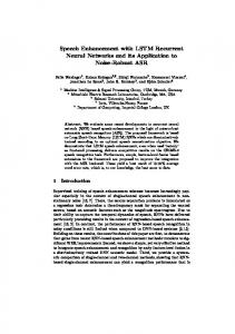
Figure 1: The general architecture of the quench detector. lowing functions (Fig. 1): • Monitoring of the voltage of superconducting elements,

RB - Main Dipole; RQ - Main Quadrupole; IT - Inner Triplet; IPQ Individually Powered Quadrupole; IPD - Individually Powered Dipole; EE - Energy Extraction; EEc - Energy Extraction by crowbar; m - number of magnets in circuits is not constant in this class of circuits.

• Extraction of the resistive part of the voltage Ures , • Generation of trigger signals in case the resistive voltage exceeds the threshold. The triggers are transmitted to other protection devices via current loops to initiate a safe shutdown of the electric circuits supplying the magnets. The method for compensation of the inductive voltage is simple in the case of a differential magnet circuit where two very similar inductances are connected in series in one circuit. However, in some LHC corrector magnet circuits, there are no reference elements available, hence the compensation of the inductive voltage by simple subtraction cannot be implemented. In such a case, Kirchhoff’s voltage law for the circuit must be solved. To satisfy timing requirements, the solution must be performed numerically (online) by means of using digital logic. Next, a quench candidate is validated as a real quench or noise. This is carried out by means of a time discriminator shown in Fig. 1. The voltage resistive component Ures must be higher than a threshold for the time interval longer than a validation time ∆tval in order to be classified as a quench. This condition is depicted in Fig. 2. The trigger signal has two important functions: the release of energy to quench heaters and an opening for an interlock loop. The goal of the quench heater is an acceleration of the propagation of the quench along a cable. It prevents local overheating (or even melting) of the quenching cable. The opening of the interlock loop is a method for an immediate transferring of the request for the termination of an operation of other LHC components.

cables used to build the magnets. Most of the highcurrent superconducting magnets used in the LHC are not self-protected and would be damaged or destroyed if they were not protected during the quench. Therefore, the quench protection system was introduced [3, 5]. The LHC Machine Protection System (MPS) comprises many subsystems. One of the subsystems is a Quench Protection System (QPS). This system consists of a Quench Detection System (QDS) and actuators which are activated once a quench is detected. A superconducting magnet has zero resistance and a relatively large inductance which is equal ≈ 100 mH in the case of main LHC dipole. When a constant current flows through the magnet, the total voltage across it, is zero. When the magnet loses its superconducting state (quench) the resistance becomes non-zero, hence, a voltage develops over the resistive part. This voltage is used to detect the quench. However, during normal operation (ramp up or down, fast power abort) a current change in the magnet generates an inductive voltage which might be well above the resistive voltage detection threshold. Therefore, the inductive voltage must be compensated in order to prevent the QDS from spurious triggering. Consequently, the most important part of the quench detector is an electronic module for extracting the resistive part of the total voltage. It is shown in Fig. 1. A quench detector is an electronic device with the fol4

Output

Hidden layer

Input

Figure 2: The principle of a quench validation by means of using a time discriminator.

Figure 3: The architecture of standard feed-forward neural network.

Voltage time series measured and extracted by the QPS system are sent over to two different storage systems. The system called the CERN Accelerator Logging Service (LS) contains low resolution data [13]. The second system, called POST_MORTEM, is dedicated to store data delivered by any equipment in the LHC whenever a trigger occurs [14].

operate directly on raw data. This makes them especially useful in applications where extracting features is very hard and even sometimes impossible. It turns out that there are many fields of applications where no experts exist who can handle feature extraction or the area is simply uncharted and we do not know whether the data contains latent patterns worth exploring [26–28]. Foundations of the most neural network architectures currently used were laid down between 1950 and 1990. For almost the last two decades researches were not able to take full advantage of these powerful models. But the whole machine learning landscape changed in early 2010, when deep learning algorithms started to achieve state-of-the-art results in a wide range of learning tasks. The breakthrough was brought about by several factors, among which computing power, huge amount of widely available data and affordable storage are considered to be the critical ones. It is worth noting that in the presence of large amount of data, the conventional linear models tend to under-fit or under-utilize computing resources. CNNs and feed-forward networks rely on the assumption of the independence of data within training and testing set as presented in Fig. 3. This means that after each training item is presented to the model, the current state of the network is lost i.e. temporal information is not taken into account in training a model. In the case of independent data, it is not an issue. But for data which contain crucial time or space relationships, it may lead to the loss of the majority of the information which is located in between steps. Additionally, feed-forward models expect a fixed length of training vectors which is not always the case, especially when dealing with time domain data. Recurrent neural networks (RNNs) are models with the ability to process sequential data one element at

3. Recurrent neural networks Recent years have witnessed a huge growth of deep learning applications and algorithms. They are powerful learning models, which achieve great successes in many fields and win multiple competitions [15]. The neural nets are capable of capturing latent content of the modeled objects in large hierarchies [16–19]. Two main branches of the neural networks are feed-forward and recurrent models. The members of the first one, of which Convolutional Neural Networks (CNN) is now the most prominent example, are usually used for processing data belonging to a spatial domain, where data occurrence in time is not important and not taken into account [16, 20, 21]. Opposed to that there are algorithms working in temporal domain, in which the information about the order of data is critical. Since quench analysis involves temporal dependencies of the examined signals we decided to focus on the neural network models that are capable of sequence processing, namely RNN, Long Short-Term Memory (LSTM) and Gated Recurrent Unit (GRU) [17, 22–24]. Currently, the LSTM is considered to be the best model [25] and it is also the most often used in applications. Therefore, we have decided to use it in our experiments. Unlike traditional models that are mostly based on hand-crafted features deep learning neural networks can 5

Output

y(t)

y(t+1)

y(t+2)

Hidden layer

h(t)

h(t+1)

h(t+2)

Input

x(t)

x(t+1)

x(t+2)

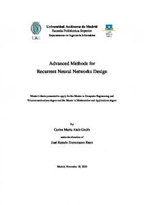
Figure 4: The general overview of recurrent neural networks. a time. Thus they can simultaneously model sequential and time dependencies on multiple scales. Unfortunately, a range of practical applications of standard RNN architectures is quite limited. This is caused by the influence of a given input on hidden and output layers during the training of the network. It either decays or blows up exponentially as it moves across recurrent connections. This effect is described as the vanishing gradient problem [17]. There had been many unsuccessful attempts to address this problem before LSTM was eventually introduced by Hochreiter and Schmidhuber [25] which ultimately solved it. Recurrent neural networks may be visualized as looped-back architectures of interconnected neurons. This was presented in Fig. 4. Originally RNNs were meant to be used with single variable signals but they have also been adapted for multiple stream inputs [17]. It is a common practice to use feed-forward network on top of recurrent layers together in order to map outputs from RNN or LSTM to the result space as presented in Fig. 5.

Output

Feed-forward layer

Hidden layer

Input

Figure 5: The mapping of outputs of a recurrent neural network. h(t)

sigm

3.1. RNN

x(t)

+

Architecture of standard neural networks is presented in Fig. 6. The nodes of the network receive input from the current data point x(t) as well as the hidden state values of the hidden layer in the previous state h(t−1) . Thus, inputs at time t have impact on the outputs of the network to come in the future by the recurrent connections. There are two fundamental equations (1) and (2), which characterize feed-forward computations of a re-

+

Standard RNN cell

h(t-1)

Sum over weighted inputs Connection to next time step

Figure 6: A cell of a standard recurrent neural network. 6

learn long-range dependencies as compared to standard RNNs. Therefore, most of state-of-the-art applications use the LSTM model [29]. The LSTM internal structure is based on a set of connected cells. The structure of one cell is presented in Fig. 7, it contains feedback connection storing the temporal state of the cell. Additionally, the LSTM cell contains three gates and two nodes which serve as an interface for information propagation within the network. There are three different gates in each LSTM cell:

hc(t) h(t-1)

oc(t)

+

sigm

x(t) sc(t) tanh

h(t-1)

• input gate i(t) c which controls input activations into the memory element,

fc(t)

+

sigm

Internal state

• output gate o(t) c controls cell outflow of activations into the rest of the network,

x(t)

• forget gate fc(t) scales the internal state of the cell before summing it with the input through the selfrecurrent connection of the cell. This enables gradual forgetting in the cell memory.

+ h(t-1)

ic(t)

+

sigm

x(t) gc(t) tanh

In addition, the LSTM cell also comprises of an input (t) node g(t) c and an internal state node sc . Modern LSTM architectures may also contain peephole connections [30]. Since they are not used in the experiment, they were neither depicted in Fig. 7 nor addressed in this description. The output of a set of LSTM cells is calculated according to the following set of vector equations:

+

LSTM cell x(t)

h(t-1)

Pointwise multiplication

+

Sum over weighted inputs Connection to next time step

Figure 7: An architecture of the LSTM cell current neural network as presented in Fig. 6. h(t) = Q(W(hx) x(t) + W(hh) h(t−1) + bh ),

(1)

yˆ (t) = so f tmax(W(yh) h(t) + by )

(2)

where: Q is an activation function. W(hx) , W(yh) and W(hh) are weights matrices of input-hidden layer, hidden-output layer and recurrent connections respectively. bh and by are vectors of biases. Standard neural networks are trained across multiple time steps using the algorithm called backpropagation through time [29].

g(t) = φ(Wgx x(t) + Wgh h(t−1) + bg ),

(3)

i(t) = σ(Wix x(t) + Wih h(t−1) + bi ),

(4)

f (t) = σ(W f x x(t) + W f h h(t−1) + b f ),

(5)

o(t) = σ(Wox x(t) + Woh h(t−1) + bo )

(6)

s(t) = g(t) i(t) + s(t−1) f (t) ,

(7)

h(t) = φ(s(t) ) o(t) .

(8)

While examining equations (3) – (8), it may be noticed that instances for a current and previous time step are used for the value of the output vector of hidden layer h as well as for the internal state vector s. Consequently, h(t) denotes a value of an output vector at the current time step, where as h(t−1) refers to the previous step. It is also worth noting that the equations contain vector notation which means that they address the whole

3.2. LSTM In practical applications, the Long Short-Term Memory (LSTM) model has shown extraordinary ability to 7

• a specific Django database back-end.

set of LSTM cells. In order to address a single cell a subscript c is used as it is presented in Fig. 7, where for instance h(t) c refers to a scalar value of an output of this particular cell. The LSTM network learns when to let an activation into the internal states of its cells and when to let an activation of the outputs. This is a gating mechanism and all the gates are considered as separate components of the LSTM cell with their own learning capability. This means that the cells adapt during training process to preserve a proper information flow throughout the network as separate units. This means that when the gates are closed, the internal cell state is not affected. In order to make this possible a hard sigmoid function σ was used, which can output 0 and 1 as given by equation (9). This means that the gates can be fully opened or fully closed.    0 if x ≤ tl ,     σ(x) =  ax + b if x ∈ (tl , th ),     1 if x ≥ th .

As the access library to CERN Oracle from Django a Python library cx_oracle [34] is used. For results capturing and maintaining appropriate data model is defined, which can be created by means of the tool called inspectdb available inside Django. Information necessary for this process is taken from database tables, however relationship between the tables should be separately defined. Dashboard for an application will be designed with widgets and plots available within ELQA framework and Bokeh library. 5. Experiments This section presents the results of the experiments which were conducted in order to validate performance of the LSTM network in an anomaly detection task. All the experiments required several steps of preparation which were mostly related to a data preprocessing.

(9)

5.1. Setup description

In terms of the backward pass, so-called constant error carousel enables the gradient to propagate back through many time steps, neither exploding nor vanishing [25, 29].

Data acquired from all the CERN accelerators are kept in the global database called Logging Service (LS) [13]. A generic Java GUI called TIMBER [35] and a dedicated Python wrapper [36] are provided as tools to visualize and extract logged data. The logging database stores a record of many years of the magnets activity. This is a huge amount of data with relatively few quench events. Therefore, the first research question that had to be addressed was related to a time span surrounding a quench event which should be taken into account for the LSTM model construction. It is worth noting that one day-long record of single voltage time series for a single magnet occupies roughly 100 MB. There are several voltage time series associated with a single magnet [35] but ultimately we decided to use Ures in our experiments. The origin and the meaning of the resistive voltage Ures were discussed in the subsection 2.2. There are various kinds of magnets located in the LHC tunnel and they generate different number of quench events (Tab. 2). It is beneficial to choose a group of magnets for which the largest possible number of quenches was recorded. The longest history of quenches was provided for 600 A magnets in LS database. Therefore, we decided to focus our initial research on 600 A magnets. Unfortunately, the 600 A magnets data stored in a database is very large i.e. an order of several gigabytes. However, as it was mentioned before, the activity record of superconducting

4. Visualization framework The model is intended to be integrated within visualisation environment for the experiments. Python framework based on Django (storing and managing experiments setup data) [31] and Bokeh (interactive Python library for visualisation of data) [32] will be used for the development of web application for quench prediction. Described LSTM model will be integrated to building blocks of an ELQA data analysis framework [33] developed at Machine Protection and Electrical Integrity group (TE-MPE) in order to prototype a web based quench prediction application for use at CERN. In the ELQA framework, an access to the data is addressed with the Object-Relational Mapping. The Django framework handles this mapping and provides full functionality of the Structure Query Language (SQL). The architecture of the Django is organized with three layers as follows: • the bottom layer which is a database, followed by • an access library that is responsible for a communication between Python and the database by means of SQL statements and 8

Quench list

Python script based on Timber API

Table 3: The data sets used for training and testing the model.

Data extraction parameters

Logging database

Voltage time series

Data set

size [MB]

small medium large

22 111 5000

frame before and after the quench events were considered. Ultimately, we chose in our view a reasonable trade-off between the amount of data and their representativeness for the model i.e. 24 hour long time window before a quench event. We extracted days on which quenches occurred between the years 2008 and 2016, which amounted to 425 in total for 600 A magnets (Tab. 2). A training of deep learning models takes long time even when fast GPUs are employed for the calculations. Therefore, it is important what kind of and how large data sets are used for training and testing the models. Furthermore, it is important to preliminary adjust hyperparameters of the model using relatively small data set when a single iteration time is short. Thereafter, tiny updates are done using the largest dataset, when each training routine of the network consumes substantial amount of time. Thus, we have created three different data sets: small, medium and the large ones as presented in Tab. 3.

Tagging

Normalization

Split of the data to Train and test set

Figure 8: The procedure for extraction of voltage time series with quench events from the LS database.

magnets during operational time of the LHC is composed mostly of sections of normal operation and only sometimes quench events happen. Furthermore, the logging database does not enable automated quench periods extraction, despite having many useful features for a data preprocessing and information extraction. It would be a tedious work to manually extract all the quenches. Therefore, a quench extraction application (presented in Fig. 8) was developed, which automates the process of fetching the voltage time series from the LS database. It is composed of a set of Python scripts which generate appropriately prepared queries to the LS database. The queries are built based on the quench list [12] and data extraction parameters configuration files. Once the data has been fetched from the LS database it is normalized to the range from 0 to 1 and split into training and testing set: 70 % of the data is used for training and 30 % for testing. Since quench events vary slightly in shape as presented in Fig. 9, they were tagged in order to make them more recognizable. What is really interesting from the perspective of the LSTM model is a time and a voltage prior to a quench event which is used for the training and prediction. Different lengths of time window

5.2. Results and analysis The designed LSTM model was examined with a respect to its ability of anticipating few voltage values forward. The core architecture of the module used for the experiments is presented in Fig. 10, but we trained and tested various models with wide range of parameters such as number of neurons, layers and inputs. The primary goal was to find a core set of the parameters which enabled unrevealing hidden trends within the Ures voltage data. The core architecture of the network module is composed of seven layers all together: an input layer, four LSTM hidden layers, one feed-forward hidden layer and an output layer. It is worth noting that dropout operations are also classified as separate layers. Every second layer among layers of the LSTM type has a dropout with a value of 20 %. Furthermore, a number of LSTM cells in the middle layer were changed from 32 to 128 and then to 512 in order to examine the performance of the model as a function of the number of neurons. The module was implemented in Keras [37] with the Theano backend [38]. 9

0.3

0.2

0.2

0.1

0.1

Voltage U_res [V]

Voltage U_res [V]

0.3

0.0 0.1 0.2

0.1 0.2

0.3 0

10

20 30 40 50 time [steps], single step: 0.4 s

60

0.3 0

70

0.3

0.3

0.2

0.2

0.1

0.1

Voltage U_res [V]

Voltage U_res [V]

0.0

0.0 0.1 0.2

10

20 30 40 50 time [steps], single step: 0.4 s

60

70

10

20 30 40 50 time [steps], single step: 0.4 s

60

70

0.0 0.1 0.2

0.3 0

10

20 30 40 50 time [steps], single step: 0.4 s

60

0.3 0

70

Figure 9: The selected sample quench events of 600 A magnets extracted from the LS database. Sample quench events are presented in Fig. 9. It may be noticed that they are similar, but some differences are noticeable. They may be considered as anomalous behavior since they do not occur often during regular operation of the LHC accelerator. As such they are very useful for the validation of the feasibility of using an LSTM model in an anomaly detection in the voltage time series of the magnets. Fig. 11 shows both real voltage signal and its prediction. Visual similarity analysis is neither efficient nor recommended for validation of regression models therefore authors have decided to use more reliable measures such as Root Mean Square Error (RMSE) and Mean Percentage Error (MPE). The measures are given by the following equations: v u t N 1 X (t) RMSE = (y − yˆ (t) )2 (10) N t=1

Output

Dense (feed-forward)

Dropout – 0.2

LSTM 32 : 512 cells

Dropout – 0.2

LSTM – 32 cells

N

Input – 1:32 steps

MPE =

100% X y(t) − yˆ (t) N t=1 y(t)

(11)

where: y(t) and yˆ (t) is a voltage time series and its predicted counterpart, respectively. Both equations (10) and (11) are calculated for N data points which in turn depend on the size of data set that is used to train and test the model.

Figure 10: The LSTM-based network used for the experiments.

10

0.8

0.7

0.7

0.6

0.6

Normalized Voltage

Normalized Voltage

0.8

0.5 0.4 0.3

0.5 0.4 0.3

0.2

0.2

0.1

0.1

0.0 0

20

40

60

time [steps], single step: 0.4 s

80

0.0 0

100

20

40

60

time [steps], single step: 0.4 s

(a) One step ahead

80

(b) Two steps ahead

Figure 11: Two examples of prediction for one and two steps ahead in time. Predicted signal is plotted in a green broken line. Table 4: The best results obtained for the medium corpus (Tab. 3).

It is worth emphasizing that in order to classify anomalies such as quenches it is essential to map regression results to classification task. In other words, it is necessary to express RMSE as given by equation (10) in terms of F1 score. Unfortunately, this requires well defined threshold of RMSE value which would discriminate positive and negative classification results. At the current stage of the research, the threshold value has not been determined and requires further investigation. Fig. 12 – 14 present the prediction results in terms of RMSE for 32 future steps. The model was trained using the medium data corpus. Two quantities were used as parameters:

LSTM cells

L

B

mean RMSE

128 32 128 32

16 1 32 1

2048 2048 128 32

0.001 04 0.001 25 0.001 40 0.001 48

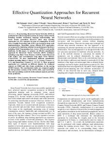
size B = 2048. In the case of the experiments with 128 neurons, the parameters combination of L = 32 and batch size B = 2048 resulted in the best result in terms of RMSE as it is presented in Fig. 13. The MPE values, according to equation (11), were computed for a selected quench fragments in parallel to the RMSE calculation of the whole voltage time series. The results of the MPE calculation generally follow the RMSE trend, therefore we decided not to include them. However, a sample MPE plot is presented in Fig. 15. It is worth noting that a prediction quality is lower for more steps ahead. This is due to the fact the a prediction of tn+1 time step is based on a previous tn step. We assumed that distortions over 25 ÷ 30 % in MPE are unacceptable and do not allow to distinguish between normal and quench behavior of an examined magnet. Tab. 4 presents the results in terms of the mean value of the RMSE. The results were obtained by averaging the RMSE error over all the steps in the future. It is worth emphasizing that the lowest RMSE error is achieved for predictions with a small number of forward steps. The more steps to the future are predicted, the worse results are obtained which is reflected in the rising RMSE value. Therefore, the results provided by Tab. 4

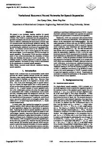
L - a number of previous time steps to use as input variables to predict the next time period, B - a size of training batch. The experiments were conducted for three different L values: 1, 16 and 32 which also affected the model input size. The more steps back in time are taken into account in model training and testing processes the wider input should be used. The size of the model input is equal to a number of steps back L in time which are taken for building the LSTM model. Furthermore, four different batch sizes B values were tested: 32, 128, 512 and 2048. The batch size B has two-fold effect on the performance of the model. On the one hand it affects a range of the voltage series which is processed by the model. On the other hand, the larger batches are computed faster on GPUs because matrix calculation optimization measures may be applied. According to Fig. 12, the best result (in terms of mean RMSE) in the experiment with 32 neurons used in the middle LSTM layer was obtained for L = 16 and batch 11

100

1

L=1, B=32 L=1, B=128 L=1, B=512

0.1

L=1, B=2048

RMSE

L=16, B=32 L=16, B=128

0.01

L=16, B=512 L=16, B=2048 L=32, B=32

0.001

L=32, B=128 L=32, B=512 L=32, B=2048

0.0001

0.00001 0

4

8

12

16

20

24

28

32

Prediction steps

Figure 12: The value of RMSE as a function of prediction steps for different batch size B and number of previous time steps L values with 32 neurons in the middle LSTM layer.

1

L=1, B=32 L=1, B=128 L=1, B=512

0.1

L=1, B=2048

RMSE

L=16, B=32 L=16, B=512

0.01

L=16, B=2048 L=32, B=32 L=32, B=128

0.001

L=32, B=512 L=32, B=2048

0.0001

0.00001 0

4

8

12

16

20

24

28

32

Prediction steps

Figure 13: The value of RMSE as a function of prediction steps for different batch size B and number of previous time steps L values with 128 neurons in the middle LSTM layer. 12

1

L=1, B=32 L=1, B=128 L=1, B=512

0.1

L=1, B=2048

RMSE

L=16, B=32 L=16, B=128

0.01

L=16, B=512

0.001

0.0001

0.00001 0

4

8

12

16

20

24

28

32

Prediction steps

Figure 14: The value of RMSE as a function of prediction steps for different batch size B and number of previous time steps L values with 512 neurons in the middle LSTM layer.

90

neurons128_lookback16_steps32_epoch6_batch2048, Mean_MPE: 64.9774954021 neurons128_lookback16_steps32_epoch6_batch32, Mean_MPE: 75.8919013739 neurons128_lookback16_steps32_epoch6_batch512, Mean_MPE: 76.3435213566 neurons128_lookback16_steps32_epoch6_batch128, Mean_MPE: 30.1802316904

80 70

mpe

60 50 40 30 20 10 0

5

10 15 20 25 prediction [time steps ahead]

30

35

Figure 15: The example of the MPE plot as a function of prediction steps for different batch size B and number of previous time steps L values. 13

rmse

10-2

corpus_large_batch_2048, Mean_RMSE: 0.000946570996844 corpus_large_batch_32, Mean_RMSE: 0.00101503350314 corpus_large_batch_512, Mean_RMSE: 0.000978525592071 corpus_large_batch_128, Mean_RMSE: 0.00114589775537

10-3

10-4 0

5

10 15 20 25 prediction [time steps ahead]

30

35

Figure 16: The example of the RMSE plot as a function of prediction steps for the large corpus (Tab. 3). Table 5: The parameters of the LSTM network used to the experiments. Parameter

Value

Number of layers Number of epochs Total number of the network parameters Dropout Max. number of steps ahead

5 6 21 025 0.2 32

were not able to conduct the same set of experiments as we did for the medium size corpus. Nevertheless, the results we managed to gather show that the RMSE value converges to a value on the level of 0.001. This was expected since much more data was used for the experiment with the large corpus. 6. Conclusions The quench events were used as an example of anomalous behavior of the superconducting magnets for the verification of an ability of using LSTM recurrent neural networks to predict anomalies. It has been proved that LSTM-based setup performs well in experiments with the data acquired from the logging database. As it was expected, prediction results for more steps ahead are inferior to the short time prediction in terms of accuracy expressed in RMSE. As a future work, the post-mortem data of much bigger resolution will be used. We are also going to implement the prediction stage of the algorithm in FPGA or ASIC to evaluate its performance in real-time applications.

should be considered as an approximate performance of the LSTM model. Nevertheless, it is noticeable that the best two results are achieved for batch size of 2048. All the tests presented in this section were performed on Intel(R) Core(TM) i7-4790 CPU @ 3.60 GHz with Radeon R9 390 STRIX GPU platform and 32 GB DDR3 1600 MHz memory. Despite using the powerful GPU, processing time is long. It took over two weeks to compute the presented results. The biggest contribution was the training time of the LSTM model, which was significantly higher for the architectures with more neurons. This was the main reason why the model was trained over only six epochs as presented in Tab. 5. A test for the large corpus (Tab. 3) of 5 GB was also conducted and an example of the results is presented in Fig. 16. Because of the long computation time we

References [1] A. Wright, R. Webb, The Large Hadron Collider, Nature 448 (7151) (2007) 269–269. doi:10.1038/448269a.

14

[2] L. Evans, P. Bryant, LHC Machine, Journal of Instrumentation 3 (08) (2008) S08001. doi:10.1088/1748-0221/3/08/ S08001. [3] R. Denz, Electronic systems for the protection of superconducting elements in the LHC, IEEE Transactions on Applied Superconductivity 16 (2) (2006) 1725–1728. doi:10.1109/ TASC.2005.864258. [4] L. Bottura, Cable stability, Proceedings of the CAS-CERN Accelerator School: Superconductivity for Accelerators, Erice, Italy (CERN-2014-005) (2014) 401–451. arXiv:1412.5373, doi:10.5170/CERN-2014-005.401. [5] A. Skoczen, J. Steckert, Design of FPGA-based Radiation Tolerant Quench Detectors for LHC, (to be published in JINST). [6] M. Calvi, L. Agrisani, L. Bottura, A. Masi, A. Siemko, On the use of wavelet transform for quench precursors characterization in the lhc superconducting dipole magnets, IEEE Transactions on Applied Superconductivity 16 (2) (2006) 1811–1814. doi: 10.1109/TASC.2006.871308. [7] C. Lorin, A. Siemko, E. Todesco, A. Verweij, Predicting the quench behavior of the lhc dipoles during commissioning, IEEE Transactions on Applied Superconductivity 20 (3) (2010) 135– 139. doi:10.1109/TASC.2010.2043076. [8] ATLAS Collaboration, Observation of a new particle in the search for the standard model higgs boson with the ATLAS detector at the LHC, Physics Letters B 716 (1) (2012) 1–29. arXiv:1207.7214, doi:10.1016/j.physletb.2012.08.020. [9] CMS Collaboration, Observation of a new boson at a mass of 125 gev with the CMS experiment at the LHC, Physics Letters B 716 (1) (2012) 30 – 61. doi:10.1016/ j.physletb.2012.08.021. [10] L. Burnod, D. Leroy, Influence of Beam Losses on the LHC Magnets, Tech. Rep. LHC-NOTE-65 (Dec 1987). URL http://cds.cern.ch/record/1017593 [11] Layout Database [online, cited 10.10.2016]. [12] Quench Database [online, cited 10.10.2016]. [13] C. Roderick, G. Kruk, L. Burdzanowski, The CERN accelerator logging service-10 years in operation: a look at the past, present and future, Proceedings of ICALEPCS2013 (2013) 612–614. URL http://cds.cern.ch/record/1611082 [14] E. Ciapala, F. RodrÃŋguez-Mateos, R. Schmidt, J. Wenninger, The LHC Post-mortem System, Tech. Rep. LHC-PROJECTNOTE-303, CERN, Geneva (Oct 2002). URL http://cds.cern.ch/record/691828 [15] A. Krizhevsky, I. Sutskever, G. E. Hinton, ImageNet Classification with Deep Convolutional Neural Networks, in: F. Pereira, C. J. C. Burges, L. Bottou, K. Q. Weinberger (Eds.), Advances in Neural Information Processing Systems 25, Curran Associates, Inc., 2012, pp. 1097–1105. URL http://papers.nips.cc/paper/4824-imagenetclassification-with-deep-convolutional-neuralnetworks.pdf [16] Y. LeCun, Y. Bengio, G. Hinton, Deep learning, Nature 521 (7553) (2015) 436–444, insight. doi:10.1038/ nature14539. [17] A. Graves, Neural Networks, Springer Berlin Heidelberg, 2012. doi:10.1007/978-3-642-24797-2. [18] J. Schmidhuber, Deep learning in neural networks: An overview, Neural Networks 61 (2015) 85 – 117. arXiv: 1404.7828, doi:10.1016/j.neunet.2014.09.003. [19] D. Y. Li Deng, Deep Learning: Methods and Applications, Tech. Rep. MSR-TR-2014-21 (May 2014). URL https://www.microsoft.com/en-us/research/ publication/deep-learning-methods-andapplications/ [20] C. Farabet, C. Couprie, L. Najman, Y. LeCun, Learning Hi-

[21]

[22]

[23]

[24]

[25]

[26]

[27]

[28]

[29]

[30]

[31] [32] [33]

[34] [35] [36] [37] [38]

15

erarchical Features for Scene Labelling, IEEE Transactions on Pattern Analysis and Machine Intelligence 35 (8) (2013) 1915– 1929. doi:10.1109/TPAMI.2012.231. Y. LeCun, Deep Learning of Convolutional Networks, in: 2015 IEEE Hot Chips 27 Symposium (HCS), 2015, pp. 1–95. doi: 10.1109/HOTCHIPS.2015.7477328. J. Morton, T. A. Wheeler, M. J. Kochenderfer, Analysis of Recurrent Neural Networks for Probabilistic Modelling of Driver Behaviour, IEEE Transactions on Intelligent Transportation Systems PP (99) (2016) 1–10. doi:10.1109/ TITS.2016.2603007. F. Pouladi, H. Salehinejad, A. M. Gilani, Recurrent Neural Networks for Sequential Phenotype Prediction in Genomics, in: 2015 International Conference on Developments of E-Systems Engineering (DeSE), 2015, pp. 225–230. doi:10.1109/ DeSE.2015.52. X. Chen, X. Liu, Y. Wang, M. J. F. Gales, P. C. Woodland, Efficient Training and Evaluation of Recurrent Neural Network Language Models for Automatic Speech Recognition, IEEE/ACM Transactions on Audio, Speech, and Language Processing 24 (11) (2016) 2146–2157. doi:10.1109/ TASLP.2016.2598304. S. Hochreiter, J. Schmidhuber, Long Short-Term Memory, Neural Comput. 9 (8) (1997) 1735–1780. doi:10.1162/ neco.1997.9.8.1735. C. Y. Chang, J. J. Li, Application of deep learning for recognizing infant cries, in: 2016 IEEE International Conference on Consumer Electronics-Taiwan (ICCE-TW), 2016, pp. 1–2. doi:10.1109/ICCE-TW.2016.7520947. M. Cai, Y. Shi, J. Liu, Deep maxout neural networks for speech recognition, in: Automatic Speech Recognition and Understanding (ASRU), 2013 IEEE Workshop on, 2013, pp. 291–296. doi:10.1109/ASRU.2013.6707745. L. Tóth, Phone recognition with deep sparse rectifier neural networks, in: 2013 IEEE International Conference on Acoustics, Speech and Signal Processing, 2013, pp. 6985–6989. doi: 10.1109/ICASSP.2013.6639016. Z. C. Lipton, J. Berkowitz, C. Elkan, A Critical Review of Recurrent Neural Networks for Sequence Learning (2015). arXiv:1506.00019. K. Greff, R. K. Srivastava, J. Koutník, B. R. Steunebrink, J. Schmidhuber, LSTM: A Search Space Odyssey (2015). arXiv:1503.04069. Django Software Foundation. Django documentation [online] (2015) [cited 10.10.2016]. Bokeh Development Team. Bokeh: Python library for interactive visualization [online] (2014) [cited 10.10.2016]. L. Barnard, M. Mertik, Usability of visualization libraries for web browsers for use in scientific analysis, International Journal of Computer Applications 121 (1). cx_Oracle [online] (2015) [cited 10.10.2016]. Logging Database TIMBER [online, cited 10.10.2016]. R. D. Maria. Python API to Timber database - pytimber [online] (2016) [cited 10.10.2016]. Deep learning library for theano and tensorflow - keras [online, cited 10.10.2016]. Theano Development Team, Theano: A Python framework for fast computation of mathematical expressions (May 2016). arXiv:1605.02688.