Non-Linear Prediction with LSTM Recurrent Neural Networks for Acoustic Novelty Detection Erik Marchi1 , Fabio Vesperini2 , Felix Weninger1 , Florian Eyben1 Stefano Squartini2 , and Bj¨orn Schuller3,4 1
2
Machine Intelligence & Signal Processing Group, TU M¨unchen, Germany A3LAB, Department of Information Engineering, Universit`a Politecnica delle Marche, Italy 3 Chair of Complex and Intelligent Systems, University of Passau, Germany 4 Department of Computing, Imperial College London, UK Email:
[email protected]
Abstract—Acoustic novelty detection aims at identifying abnormal/novel acoustic signals which differ from the reference/normal data that the system was trained with. In this paper we present a novel approach based on non-linear predictive denoising autoencoders. In our approach, auditory spectral features of the next short-term frame are predicted from the previous frames by means of Long-Short Term Memory (LSTM) recurrent denoising autoencoders. We show that this yields an effective generative model for audio. The reconstruction error between the input and the output of the autoencoder is used as activation signal to detect novel events. The autoencoder is trained on a public database which contains recordings of typical in-home situations such as talking, watching television, playing and eating. The evaluation was performed on more than 260 different abnormal events. We compare results with stateof-the-art methods and we conclude that our novel approach significantly outperforms existing methods by achieving up to 94.4 % F-Measure.
I.
I NTRODUCTION
Novelty detection is a challenging task, and it aims at recognising situations in which unusual events occur. The problem can be treated as one-class classification task: typically the amount of normal data consists of a very large set, and the normal class can be accurately modelled, whereas the acoustic events belonging to the class are considered novel events. Many approaches have been proposed due to the practical importance of the novelty detection, especially for automatic monitoring systems. In the past years, many systems have been deployed for surveillance applications. Surveillance can be seen as control of public safety or as the supervision of private environments where people may live alone. In fact, the increasing requirement of public security over the past decades has motivated the installation of sensors such as cameras or microphones in public places (stores, subway, airports, etc.). Thus, the need of unsupervised situation assessment stimulated the signal processing community towards experimenting with several automated frameworks. Usually, the research in the area of automatic surveillance systems is mainly focused on detecting abnormal events based on the acquired video information. Anyway, the information given by the acoustic signal offers several advantages, such as low computational needs or the fact that the illumination conditions of the space to be monitored do not have an immediate effect on sound; the same applies for possible
occlusion or fast events like shots or explosions. The statistical approach is the most widely used for this problem. Its principle is to model data based on its statistical properties and using this information to estimate whether a test sample comes from the same distribution or not. A. Related work Statistical and probabilistic approaches are the most commonly used in the field of novelty detection. Novelty detection ranges from automatic recognition of handwriting, the recognition of cancer [1], informatic intrusion detection systems, non-destructive inspection for the analysis of mechanical components [2], audio segmentation [3], to many others. As early as in 1994, a pioneering study investigated the relationship between the degree of novelty of the input data and the corresponding reliability of the outputs from the neural network, and demonstrated its performance using an application on the control of the oil flow in multiphases pipelines [4]. Subsequent works proposed the application of a compression autoencoder neural network to detect abnormal CPU data usage [5], [6]. In further works [7], [8], [9], [10], the use of a compression autoencoder for outlier detection was studied and in [11] the autoencoder was applied for the task of damage classification under changing environmental conditions. A technique based on a neural network with the task of classifying mixed acoustic events is presented in [12]. The system uses a feed-forward network and splits the input signals into classes or novelty events; it has been tested in a real underwater environment and realises the detection of recurrent events. Overall, several studies exists in the field of acoustic event classification applying Gaussian Mixture Models (GMMs) and Hidden Markov Models (HMMs) to detect human presence (speech, laughter, cough), animal sounds, sounds of objects [13], [14] and sounds caused by various types of guns [15]. However, it is to be emphasised that there is a fundamental difference between event classification and novelty detection: the latter has the greater difficulty of not having a priori knowledge of any element of the novelty class. It can be argued that this makes generative models, such as GMMs and HMMs, particularly suited for this task. For example, studies investigated HMM- and GMM-based approaches for acoustic surveillance of abnormal situations [16], [17] and for automatic space monitoring [18]. A (pseudo-)generative
model for acoustic novelty detection in the form of a denoising autoencoder has been introduced in a recent study [19]. B. Contribution A novel weakly supervised method based on a non-linear prediction denoising autoencoder with LSTM recurrent neural networks is introduced for novelty acoustic detection. The use of LSTM as generative model [20] for text [21], handwriting [21], and music [22] generation was recently investigated, however – to our best knowledge – the use of LSTM as a model for audio generation is novel. In our approach the LSTM are trained to predict next frames from previous ones. The auditory spectral features are processed by the autoencoder, which acts as a one-class classifier. Our approach relies on the reconstruction error which the denoising autoencoder commits trying to predict and reconstruct a novel sound which the network has never seen in the training phase. We compare results with state-of-the-art methods and we conclude that our improved approach significantly outperforms existing methods by achieving up to 94.4 % F -Measure. This contribution is structured as follows: First, a basic description of the different autoencoder-based schemes for acoustic novelty detection is given (Section II), together with the presentation of the non-linear prediction approach. Then the LSTM recurrent neural networks, thresholding strategy, and features employed in experiments are described in Section III. The used database and the experimental set-up are jointly discussed with the evaluation of obtained results in Section IV. Section V finally draws the paper conclusions.
Given an input set of examples X , autoencoder training consists in finding parameters θ = {W1 , W2 , b1 , b2 } that minimise the reconstruction error, which corresponds to minimising the following objective function: X 2 J (θ) = kx − x ˜k . (3) x∈X
The minimization is usually realised by stochastic gradient descent as in the training of neural networks. The structure of the AE is given in Figure 1a. B. Compression Autoencoder In the case of having the number of hidden units m smaller than the number of input units n, the network is forced to learn a compressed representation of the input. For example, if some of the input features are correlated, then this Compression Autoencoder (CAE) is able to learn those correlations and reconstruct the input data from a compressed representation. The structure of the AE is given in Figure 1b. C. Denoising Autoencoder The denoising autoencoder [25] forces the hidden layer to retrieve more robust features and prevent it from simply learning the identity. In such a configuration the autoencoder is trained to reconstruct the input from a corrupted version of it. Formally, the initial input x is corrupted by means of additive isotropic Gaussian noise in order to obtain: x0 |x ∼ N (x, σ 2 I). The corrupted input x0 is then mapped, as with the basic autoencoder, to a hidden representation h(x0 ) = f (W10 x0 + b01 ),
II.
AUTOENCODERS FOR ACOUSTIC N OVELTY D ETECTION
from which we reconstruct a the original signal as follows
This section introduces the basic concepts of autoencoders and describes the basic autoencoder, compression autoencoder, denoising autoencoder, and non-linear predictive autoencoder. A. Basic Autoencoder A basic autoencoder (AE) – a kind of neural network typically consisting of only one hidden layer –, sets the target values to be equal to the input. Deep neural networks use it, as an element, to find common data representation from the input [23], [24]. Formally, in response to an input example x ∈ Rn , the hidden representation h(x) ∈ Rm is h(x) = f (W1 x + b1 ),
(1)
where f (z) is a non-linear activation function, typically a logistic sigmoid function f (z) = 1/(1 + exp(−z)) applied component-wise, W1 ∈ Rm×n is a weight matrix, and b1 ∈ Rm is a bias vector. The network output maps the hidden representation h back to a reconstruction x ˜ ∈ Rn : x ˜ = f (W2 h(x) + b2 ),
(4)
(2)
where W2 ∈ Rn×m is a weight matrix, and b2 ∈ Rn is a bias vector.
x ˜0 = f (W20 x + b02 ).
(5)
The parameters θ0 = {W10 , W20 , b01 , b02 } are trained to minimise the average reconstruction error over the training set, to have x ˜0 as close as possible to the uncorrupted input x, which corresponds to minimising the objective function in Equation 3. The structure of the denoising autoencoder is shown in Figure 1c. D. Non-Linear Predictive Autoencoder The idea of a non-linear predictive autoencoder is quite intuitive. The autoencoder is trained to predict the next frame from the previous one. Formally, the input up to a given time frame xt is mapped to a hidden representation h h(xt ) = f (W1∗ , b∗1 , x1,...,t ),
(6)
where W and b denote weights and bias, respectively. From this we reconstruct an approximation of the original signal as follows, x ˜t+k = f (W2∗ , b∗2 , h1,...,t ), (7) where k is the prediction delay, and hi = h(xi ). The parameters θ∗ = {W1∗ , W2∗ , b∗1 , b∗2 } are trained to minimise the average reconstruction error over the training set, to have x ˜t+k as close as possible to the prediction delay. A prediction delay of k = 1 corresponds to a shift of 10 ms in the audio signal (cf.
{˜ x:x ˜ ∈ Xtr , Xte }
{˜ x:x ˜ ∈ Xtr , Xte }
{˜ x0 : x ˜0 ∈ Xtr , Xte }
{x : x ∈ Xtr , Xte }
{x : x ∈ Xtr , Xte }
{x0 : x0 ∈ Xtr , Xte }
Output layer
Hidden layer
Input layer (a)
(b)
(c)
Fig. 1. Structure of the (a) basic autoencoder (AE), (b) compression autoencoder (CAE), and (c) denoising autoencoder (DAE) on the training set Xtr or testing set Xte . Xtr contains data of non-novel acoustic events; Xte consists of novel and non-novel acoustic events.
Section III-C). The training of the parameters is performed by minimising the objective function (3) – the difference is that x ˜ is now based on non-linear prediction according to (6) and (7). The training set Xtr consists of background environmental sounds, and the test set Xte consists of recordings containing abnormal sounds. In our approach, the initial input xt is corrupted by means of additive isotropic Gaussian noise in order to obtain: x0 |x ∼ N (x, σ 2 I). The resulting structure of the non-linear predictive denoising autoencoder (NP-DAE) is shown in Figure 2. An overall block diagram of the proposed novelty detector is depicted in Figure 3. In our study, the equations (6) and (7) are implemented as LSTM-RNNs (cf. below). III.
LSTM RECURRENT NEURAL NETWORKS , THRESHOLDING , AND FEATURES
This section introduces the LSTM recurrent neural networks, describes the thresholding strategy, and the features employed in our experiments. A. LSTM LSTM networks were introduced in [26]. Compared to a conventional RNN, the hidden units are replaced by so-called {˜ x0t+k
:
x ˜0t+k
∈ Xtr , Xte }
Output layer
memory blocks. These memory blocks can store information in the cell variable ct . In this way, the network can exploit long-range temporal context. Each memory block consists of a memory cell and three gates: the input gate, output gate, and forget gate, as depicted in Fig. 4. These gates control the behaviour of the memory block. The forget gate can reset the cell variable which leads to ‘forgetting’ the stored input ct , while the input and output gates are responsible for reading input from xt and writing output to ht , respectively: ct = f t ⊗ ct−1 + it ⊗ tanh(W xc xt + W hc ht−1 + bc ) (8) ht = ot ⊗ tanh(ct )
(9)
where ⊗ denotes element-wise multiplication and tanh is also applied in an element-wise fashion. The variables it , ot and f t are the output of the input gates, output gates and forget gates, respectively, bc is a bias term, and W is the weight matrix. Each memory block can be regarded as a separate, independent unit. Therefore, the activation vectors it , ot , f t , and ct are all of same size as ht , i. e., the number of memory blocks in the hidden layer. Furthermore, the weight matrices from the cells to the gates are diagonal, which means that each gate is only dependent on the cell within the same memory block. In addition to LSTM memory blocks, we use bidirectional RNNs [27]. A bidirectional RNN can access context from both temporal directions. This is achieved by processing the input data in both directions with two separate hidden layers. Both hidden layers are then fed to the output layer. The combination of bidirectional RNNs and LSTM memory blocks leads to
Hidden layer
Input layer {x0t : x0t ∈ Xtr , Xte } Fig. 2. Structure of the non-linear predicting denoising autoencoder (NPDAE) on the training set Xtr or testing set Xte . Xtr contains data of non-novel acoustic events; Xte consists of novel and non-novel acoustic events.
Fig. 3. Block diagram of the proposed acoustic novelty detector with a denoising autoencoder. Features are extracted from the input signal and the reconstruction error between the input and the reconstructed features is then processed by a thresholding block which detects the novel or non-novel event.
ht bo
ot bf
output gate
T T
ft
xt ht1
ct
ht1
cell
forget gate
bi
T
it input gate ht1 xt
xt
xt ht1
bc
Fig. 4. Long Short-Term Memory block, containing a memory cell and the input, output, and forget gates
bidirectional LSTM networks [28], where context from both temporal directions is exploited. It has to be noted that, using bidirectional LSTM networks makes it impossible to use the system for online processing. A network composed of more than one hidden layer is referred to as a deep neural network (DNN) [29]. By stacking multiple (potentially pre-trained, but not in our system) hidden layers on top of each other, increasingly higher level representations of the input data are created (deep learning). When multiple hidden layers are employed, the output of the network is (in the case of a bidirectional RNN) computed as ←
→
yt = W →
→ hN y
hN t +W
← hN y
hN t + by ,
(10)
←
N where hN t and ht are the forward and backward activations of the N -th (last) hidden layer, respectively.
We conducted several preliminary evaluations to find the best network layout by varying the number of hidden layers and their size (i. e., the number of LSTM units for each layer). The best network layout for RNN has three hidden layers with 216 LSTM units each. The best network layout for bidirectional LSTM (BLSTM) has six hidden layers (three for each direction) with 156, 256, and 156 LSTM units respectively. Supervised learning was applied up to 100 epochs for training the network. Network weights are recursively updated by standard gradient descent with backpropagation of the sum squared error. The gradient descent algorithm requires the network weights to be initialised with non zero values; thus, we initialise the weights with a random Gaussian distribution with mean 0 and standard deviation 0.1. B. Thresholding The input and output layer of the network have 54 units. Thus, the trained autencoder is able to reconstruct each sample and novel events are identified by processing the reconstruction error with an adaptive threshold. The input x is segmented into sequences of 30 seconds of length. For every time-step the Euclidean distance between each standardised input feature value and the networks output is computed. The distances are
Fig. 5. (a): Spectrogram of a 30 seconds sequence containing three novel events, such as a siren and two screams. (b): Reconstruction error signal of the related sequence obtained with a BLSTM-DAE. (c): Reconstruction error signal of the related sequence obtanined with a non-linear predictive BLSTM-DAE (NP-BLSTM-DAE) with a prediction delay of 3 frames. (d): Reconstruction error signal of the related sequence obtanined with a NPBLSTM-DAE with a delay of 5 frames.
summed up and divided by the number of coefficients in order to represent the reconstruction error of each time-step with a single value. A threshold θth is then applied to obtain a binary signal. The threshold is shifted from the median of the error signal of a sequence e0 by a multiplicative coefficient β, which ranges from βmin = 1 to βmax = 2: θth = β ∗ median(e0 (1), ..., e0 (N ))
(11)
Fig. 5 shows the reconstruction error for a given sequence. The figure clearly depicts a low reconstruction error in reproducing normal input such as talking, television sounds, and other normal environmental sounds. On the other hand, the denoising autoencoder shows a high reconstruction error when it comes to reproduce novel acoustic events such as a scream, or an alarm. Additionally it shows how the different prediction delays modify the activation. TABLE I. ACOUSTIC NOVEL EVENTS IN THE TEST SET. S HOWN ARE THE NUMBER OF DIFFERENT EVENTS , THE AVERAGE DURATION , AND THE TOTAL DURATION IN SECONDS PER EVENT TYPE . Type
# Events
Avg. Duration (s)
Total Duration (s)
Alarm
76
6.0
435.8
Scream
111
1.9
214.6
Falls
48
1.8
89.5
Fracture
32
2.2
70.4
Total
267
2.4
810.3
C. Features Auditory Spectral Features (ASF) [30] are computed by applying Short Time Fourier Transform (STFT) using a frame
size of 30 ms and a frame step of 10 ms. Each STFT yields the power spectrogram which is converted to the Mel-Frequency scale using a filter-bank with 26 triangular filters obtaining the Mel spectrograms M30 (n, m), with n being the frame index, and m the frequency bin index. Finally, to match the human perception of loudness, a logarithmic representation is chosen: 30 Mlog (n, m) = log(M30 (n, m) + 1.0)
(12)
In addition the positive first order differences D30 (n, m) are calculated from each Mel spectrogram following: 30 30 D30 (n, m) = Mlog (n, m) − Mlog (n − 1, m)
B EST SETUPS FOR NON - LINEAR PREDICTION (NP) AUTOENCODERS IN THE DIFFERENT LAYOUTS : COMPRESSION AUTOENCODER (CAE) WITH (B)LSTM, BASIC AUTOENCODER (AE) WITH (B)LSTM, AND DENOISING AUTOENCODER (DAE) WITH (B)LSTM. Method NP-LSTM-CAE NP-BLSTM-CAE NP-LSTM-AE NP-BLSTM-AE NP-LSTM-DAE NP-BLSTM-DAE
Layout
Delay (k)
P (%)
R (%)
F1 (%)
54-30-54 54-30-54 54-54-54 54-54-54 216-216-216 156-256-156
1 3 1 2 1 3
93.7 94.6 92.5 95.7 95.2 94.9
91.3 91.1 91.6 92.5 93.2 93.9
92.5 92.8 92.1 94.1 94.2 94.4
(13)
Furthermore, the frame energy and its derivative are also included as feature ending up in a total number of 54 features. The features are extracted with our open-source audio analysis toolkit openSMILE [31]. IV.
TABLE II.
E XPERIMENTS AND R ESULTS
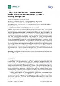
This section contains the data set used for our evaluation (Section IV-A), the experiments’ setup (Section IV-B), and a description of the performances obtained with the proposed approach (Section IV-C). A. Evaluation Data Set Our evaluation dataset is composed by around three hours of recordings of a home environment, taken from the PASCAL CHiME speech separation and recognition challenge dataset [32]. It consists of a typical in-home scenario (a living room), recorded during different days and times, while the inhabitants (two adults and two children) perform common actions, such as talking, watching television, playing, eating. We used randomly chosen sequences to compose 100 minutes of background for training set, and around 70 minutes for testing set. The original dataset was recorded in 2 channels (with a binaural microphone) and a sample-rate of 16 kHz. The test set1 was generated adding different kinds of sounds2 , such as screams, alarms, falls and fractures (cf. Table I). The test set did not include any overlapping events, the events were normalised to the volume of the background recordings, and they were added at random position thus the distance between one event and another is not fixed. B. Experimental Setup Several experiments were conducted, to find the the most suitable setup. The networks were trained with gradient steepest descent algorithm on the sum of squared errors (SSE) with a fixed momentum of 0.9, at different constant values of learning rate l = {1e−4 , 1e−5 , ..., 1e−8 }, and different noise sigma values σ = {0.01, 0.1, 0.25}. In the case of the basic (AE) and the compression autoencoder (CAE) with BLSTM and LSTM no additive Gaussian noise was applied. The prediction delay was applied at different values: k = {1, 2, 3, 4, 5, ..., 10}. One prediction delay unit corresponds to 10 ms. The autoencoders were trained using our open-source CUDA RecurREnt Neural Network Toolkit (CURRENNT) [33]. As evaluation metrics we used Precision, Recall, and F-measure. We evaluated several 1 available for download here: http://a3lab.dii.univpm.it/webdav/audio/ testset PASCAL CHiME plus novel.tar.gz 2 taken from www.freesound.org
topologies for the non-linear predictive denoising autoencoder ranging from 54-128-54 to 270-370-270, and from 54-20-54 to 54-54-54 in the case of compression/basic autoencoder. Every network topology was evaluated for each 100 epochs of training. In order to compare our results with the state of the art methods, we reported the performances obtained with normal basic, compression, and denoising autoencoders [19]. We employed further two typical approaches based on GMM and HMM. In the case of GMMs, models were trained at different numbers of Gaussian components 2n with n = {1, 2, ..., 8}, whereas left-right HMMs were trained with different numbers of states s = {3, 4, 5} and 2n Gaussian components with n = {1, 2, ..., 7}. GMMs and HMMs were trained using the Torch [34] toolkit. The log-likelihood signal produced as output of the probabilistic models was postprocessed with a similar thresholding algorithm (cf. Section III) in order to fairly compare the performances among the different methods. For all the experiments and settings we maintained the same feature set. C. Results Figure 6 reports performances for progressive values of the prediction delay (k) – from 0 up to 10 – using a Compression Autoencoder (CAE), Basic Autoencoder (AE), and Denoising Autoencoder (DAE) with both, LSTM and BLSTM neural networks. We evaluated several layouts (cf. Section IV-B) per network type, but we show only the best ones. Setting a prediction delay of 3 frames, which corresponds to a total prediction delay of 30 ms, leads to the best performances of up to 94.4 % F -Measure in the NP-BLSTM-DAE network, whereas for NP-LSTM-DAE we observe better performances with a delay of one frame (10 ms) of up to 94.2 % F -Measure (cf. Table II). For all the approaches best values of F -Measure is obtained with k = 2 or k = 3. It must be observed that, increasing the prediction delay led to a significant decrease of an F -Measure down to 86 2%. This is due to the fact that, in presence of higher prediction delays, quick periodic events induce a higher reconstruction error, as shown in Fig. 5, where the activation in subplot c clearly presents higher errors with respect to the one depicted in in subplot d. Table II reports the best results for each autoencoder type and networks. In general, the superiority of DAE schemes with respect to the CAE/AE ones is motivated by the the strength of a denoising autoencoder of encoding the input by preserving the information about the input itself and simultaneously reversing the effect of a corruption process applied to the input of the auto-encoder: The combination of these two learning
processes proved to be effective in the experimental results. Here, we combined the ability of the denoising autencoder with the non-linear prediction, allowing us to achieve the best performance (up to 94.4 % F -Measure). As an overall evaluation on the test set, Fig. 7 shows the comparison between state-of-the-art methods and our proposed approach in terms of F -Measure, Precision, and Recall. We observe that, the proposed NP-BLSTM-DAE method provided the best performance in terms of Precision, Recall, and F Measure of up to 94.9 %, 93.9 %, and 94.4 % respectively (cf. Table III). A significant absolute improvement (one-tailed ztest [35], p