A Unifying Criterion for Blind Source Separation and Decorrelation ...

A Unifying Criterion for Blind Source Separation and Decorrelation: Simultaneous Diagonalization of Correlation Matrices Hsiao-Chun Wu, Jose C. Principe Computational Neuro-Engineering Laboratory Department of Electrical and Computer Engineering University of Florida, Gainesville, FL 32611 {principe, wu}@cnel.ufl.edu

Abstract Blind source separation and blind output decorrelation are two well-known problems in signal processing. For instantaneous mixtures, blind source separation is equivalent to a generalized eigen-decomposition, while blind output decorrelation can be considered as an iterative method of output orthogonalization. We propose a steepest descent procedure on a new cost function based on the Frobenius norm which measures the diagonalization of correlation matrices to perform blind source separation as well as blind decorrelation. The method is applicable to both stationary and nonstationary signals and instantaneous as well as convolutive mixture models. Simulation results by Monte Carlo trials are provided to show the consistent performance of the proposed algorithm.

1. Introduction The field of blind signal processing which includes blind source separation, blind decorrelation and blind equalization has recently received a lot of attention. Most of the blind separation algorithms are based on high-order statistical information because it can be shown that second order statistics are not sufficient to uniquely separate sources [15]. However, this proof requires signal stationarity which is not applicable to many important real life problems (such as separation of speech). There have been also reports showing experimentally that systems based on second order statistics can indeed separate mixed sources [1]-[9]. These methods explore the time characteristics of the covariance, i.e. either nonstationary temporal estimates of covariance matrices or time-delayed cross-correlation matrices. Blind decorrelation can be formulated with second order statistics and can be solved by the orthogonalization of covariance matrices [11, 12]. Therefore methods based on second order statistics for blind source separation are related to blind decorrelation, but there is no systematic coverage of the two areas. In this paper, we will unify the

framework of blind source separation using second order statistics with blind decorrelation and apply the new algorithm to speech data. The signal separation and decorrelation problems can be modeled as X ( t ) = xk ( t ) =

∑ aki si ( t ) = AS ( t )

(1)

i

where S(t) is an N by 1 zero-mean vector containing the original signal, X(t) is an M by 1 coupled signal vector (M >= N), A is an M by N real time-invariant coupling matrix, si(t) is the ith unknown signal and aki is a real unknown coupling coefficient. If A is full rank, we can always use PCA to find the subspace of X(t) which is equivalent to the space of S(t). The objective of blind decorrelation is to design a full-rank weight matrix W that constructs an output Y(t) = WTX(t) displaying a diagonal output covariance E{Y(t)YT(t)}. However, blind separation has a different objective since one needs to design a signal separator W which is able to reconstruct the original signals. The latter constraint will put a stronger requirement on the weight matrix W such that W

T

= A –1

or

T

W A = PD

(2)

where P is a permutation matrix, D is a diagonal scaling matrix and T denotes matrix transpose [13]. The weight matrices for blind separation belong to a subset of the blind decorrelation solution.

2. Approach and criterion According to [4, 5], blind separation of nonstationary signals can be formulated as the simultaneous diagonalization of two covariance matrices estimated at different times, which can be further reduced to a generalized eigen-decomposition problem (requiring off-line processing). Orthogonalization of covariance estimates at many time instants with regularization was suggested in [6] as an on-line algorithm for blind separation. However, the method can only decorrelate signals with positivedefinite covariance matrices due to a restriction placed on the cost function. Instead of using different covariance estimates at different time intervals, one can still perform blind separation (decorrelation) through the simultaneous orthogonalization of two or more time-delayed correlation matrices [7, 8] as T

T

W E { X ( t )X ( t – q ) }W = D ( q )

(3)

where D(q) is a diagonal matrix associated with a delay q. The non-symmetrical time delayed correlation matrix E{X(t)XT(t-q)} is not necessarily positive-definite and hence we cannot apply the criterion proposed by [6]. To our knowledge only

the generalized eigen-decomposition was proposed to solve this formulation but the method is an analytic solution [7, 8]. Here we will propose an alternative criterion to solve the realistic case of non-positive-definite time-delayed correlation matrices iteratively. The idea is to create a cost function which minimizes directly the difference between the quadratic form in the left side of Eq. (3) and its right side. In order to measure the distance between the correlation estimate E{X(t)XT(t-q)} and its diagonal version, Dq(t) we propose the following criterion: d

d

2 T W T E { X ( t )X ( t – q ) }W – D q ( t )

∑ Jq( t ) = ∑

F

q=0

q=0

(4)

2

T

as well as J q ( t ) = W T E { X ( t )X ( t – q ) }W – D q ( t ) F

(5)

where F denotes the Frobenius norm and d is the total number of the delayed covariance matrices Dq(t) we need to constrain. However the choice of d still needs to be further analyzed. The Frobenius norm is defined as [14]: m n

A F =

∑ ∑ aij

2

(6)

i j

where A is an m-by-n matrix. The minimum of this cost function preserves the diagonal elements of E{X(t)XT(t-q)} but zeros all other elements out, i.e., it solves both the blind separation and decorrelation problems. The cost function of Equation (4) is a nonnegative fourth-order function of the weight coefficients W. The minimum d

can be obtained using a gradient descent procedure ∆W = – η

dJ ( t )

q - . Simple ∑ -------------dW

q=0

linear algebra manipulations yield d

∑ { [ C q ( t ) + C qT ( t ) ] W [ W T C q ( t )W – D q ( t ) ] }

∆W = – η

(7)

q=0

where

T

C q ( t ) = E { X ( t )X ( t – q ) }

(8)

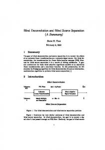
In addition, the gradient descent procedure using our proposed criterion will move the directions of the output signals in such a way that orthogonalizes all the vectors in tandem as depicted in Figure 1. This methodology is different from GramSchmidt where the principal component must stabilize before the others converge since they are corrected with respect to it. (yielding what is called the deflation procedure.) Deflation procedures converge sequentially which is a known problem for

the recent prevalent orthogonalization procedures based on the L2 norm or Rayleigh quotient optimization. ∆yi(n) yi(n+1) yi(n) yj(n) yj(n+1)

∆yj(n)

Figure 1. Illustration of orthogonalization procedure

Our procedure does not constrain the size of the vectors, so null vectors can occur during learning. This corresponds to a trivial solution that meets the minimization of the criterion of Eq. (4). To avoid it, we have to impose a unit length constraint on the weight vectors.

3. Implications of the new criterion For the case Dq(t) = I and q = 0, Eq. (7) yields, T

T

W ( t + 1 ) = W ( t ) – ηW ( t )E { Y ( t )Y ( t ) } [ E { Y ( t )Y ( t ) } – I ]

(9)

We will show that this adaptation rule was previously utilized in blind decorrelation and independent component analysis. 3.1 Stochastic Whitening Procedure If the requirement is to obtain whitened outputs, we have to estimate E{Y(t)YT(t)} either using an exponential window or batch mode. In [12] the following on-line stochastic whitening procedure was derived through a Gram-Schmidt-like orthogonalization, T

W ( t + 1 ) = W ( t ) – ηW ( t ) [ Y ( t )Y ( t ) – I ]

(10)

which is equivalent to Eq. (9) if the first E{y(t)yT(t)} is dropped. 3.2 Kullback-Leibler Divergence If we replace Y(t) by f(Y(t)) in Eq. (10), where f(*) is a proper nonlinear function,

we obtain the update rule derived from minimization of Kullback-Leibler divergence in [10]. 3. 3 Generalized Blind Decorrelation Rule The adaptation rule for generalized decorrelation at iteration n using Eq. (7) with an arbitrary square matrix Cq(t) is W n + 1 = W n + ∆W n

subject to wTn(i)wn(i) = 1, for all i =1, 2, ..., N.

(11)

where wn(i) is the ith column vector of Wn. With Eq. (11), we can extend the solution presented in [11] to any time-delayed correlation matrix. If we orthogonalize several time-delayed matrices using this procedure, we can obtain separated signals as in [7]. 3.4 On-line Adaptation Rule for Blind Separation of Nonstationary Signals (Instantaneous mixture) It has been proved in [6] that, for linear time-invariant instantaneous mixture of locally stationary signals, the source signals can uniquely be determined from the sensed signals (except the arbitrariness of the permutation matrix P and the diagonal matrix D) if and only if Eq. (12) holds E { y i ( t )y j ( t ) } = 0

for

all

i≠j

at any instant of time t. (12)

Eq. (12) can be easily translated as the orthogonalization of the output correlation matrix at any instant of time t as in Eq. (13) T

W T E { X ( t )X ( t ) }W = D 0 ( t )

at any instant of time t.

(13)

Here we propose to use batch learning with non-overlap windowed estimates. The blind source separation rule for nonstationary signals becomes for the mth batch Wm+1 = Wm + ∆Wm, subject to wTm(i)wm(i) = 1, for all i =1, 2, ..., N. where wm(i) is the ith column vector of Wm. C0 (m) has to be used in Eq. (7) to calculate ∆Wm.

4. Blind source separation of linear convolutive mixture If we have the sensed signal X(t) = [x1(t) x2(t), ..., xN(t)]T, composed by a linear

convolutive mixture of sources, X(z) = H(z)S(z), where

H(z) =

h 11 ( z )

…

h1N ( z )

…

h ij ( z )

…

h N1 ( z )

…

h NN ( z )

s1 ( z ) S( z) =

… sN ( z )

The solution Y(z) for separated signals is Y(z) = PK(z)H-1(z) where P is a permutation matrix and K(z) is a diagonal matrix with some arbitrary shaping filters as its diagonal elements. We can modify Eq. (8) as C q ( t ) = E { X ( t )X ( t – q ) }

(14)

where X ( t ) is T

. X ( t ) = [ x 1 x 2 …x N ] ; x j = [ x j ( t )x j ( t – 1 )…x j ( t – L + 1 ) ] 1≤j≤N

(15)

In addition, we also need to modify the separation weight matrix W as w 11 w 21 … w N1 W =

w 12 w 22 … w N2 …

(16)

… w ij …

w 1N w 2N … w NN T

where w ij = [ w ij ( 0 ), w ij ( 1 ), …, w ij ( L – 1 ) ] 1 ≤ i, j ≤ N is the separating filter of length L. With the new definitions of Eq. (14), (15) and (16), we can apply Eq. (7) to solve for linear convolutive mixture.

5. Simulation results Since the solution for blind source separation is a subset of blindly decorrelated outputs we focus our first experiment on blind source separation of instantaneous mixed signals. We select speech signals spoken by two male speakers (TIMIT database), and we artificially mix them with a matrix A. We acknowledge that this a simplified problem, but it is one where we have control of the experiments to test the new algorithm. The method can be easily extended to any N by N case. We choose the mixing matrix A randomly and average the performance by sixty Monte Carlo trials with sixty different random initial weights. Then we run the experiments for 200 epochs according to our proposed adaptation rule. We seek with this experiment to find how reliable is the method, i.e. how many times the

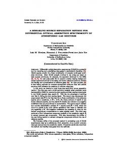
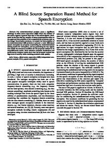
solution is found and what is the variance in the estimates. Figure 2 and 3 plot the mean Frobenius distances given by Eq. 4 versus epoch number with the corresponding one standard deviation errorbars (upper / lower limits of performance curves). In Figure 2 the criterion is J0 and all the Monte Carlo runs converged to the true solution in less than 20 epochs. On the other hand, Figure 3 shows the fast convergence of our algorithm when we try to minimize the combined criterion 3

∑ J q . Among the trials we select one to illustrate the convergence results. The q=0

particular instantaneous mixture matrix was A =

0.7012 0.7622 0.9103 0.2625

(17)

After only 4 to 12 learning epochs, the system reaches the optimization with the separation weight matrix Wopt. We can investigate if the product of two matrices WTA is actually in the form of PD as previously described [13]. Consequently we normalize each row of the product matrix WTopt A by the absolute value of its dominant element and the product as – 0.0025 – 1.0000 1.0000 0.0055

T A = W opt

(18)

From Eq. (15) we can see that we have really removed almost all the interference from the other source in this trial picked at random. From Eq. (18) we can see that SNR (signal-to-noise ratio) is 52.04 dB at receiver 1 and 45.19 dB at receiver 2 respectively. The distortion is almost unnoticeable. In our second experiment, for a convolutive mixture of two sources, we choose an arbitrary mixing matrix 1

H(z) = 0.7z

–1

+ 0.4z

0.85z

–2

+ 0.25z

–3

–2

+ 0.1z

–3

(19)

1

The algorithm needs approximately 150 epochs to converge as shown by the learning curve plotted in Figure 4 (L = 6 in Eq. (15), d = 20 in Eq. (4) and the energy of s1(t) and s2(t) are equal for this case). Since the convolutive model is more complicated we cannot simply apply the product in Eq. (18) to investigate the simulation result. However we can compute the output as T

Y ( z ) = W ( z )H ( z )S ( z ) =

ϖ 11 ( z )

…

ϖ N1 ( z )

…

ϖ ij ( z )

…

ϖ 1N ( z )

…

ϖ NN ( z )

T

H ( z )S ( z ) .

(20)

where ϖ ij ( z ) is the z-transform of w for 1 ≤ i, j ≤ N , and H(z), S(z) were previously defined. Hence from Eq. (20) the outputs for the simulation of the convolutive model can be obtained as Y i ( z ) = α i1 ( z )S 1 ( z ) + α i2 ( z )S 2 ( z ) for i = 1, 2.

(21)

or y i ( t ) = y i1 ( t ) + y i2 ( t ) where yij(t) is the inverse z-transform of α ij ( z )S j ( z ) . According to Eq. (21) the energy matrix can be defined as [8] 2

2

∑ y 11 ( t ) ∑ y 12 ( t )

0.0776 1.1534 t and it is in our simulation. 2 2 1.0787 0.0946 ∑ y 21 ( t ) ∑ y 22 ( t ) t t t

(22)

The SNR are 14.86 dB at receiver 1 and 11.40 dB at receiver 2 respectively, which is reasonable for the size of the filters employed. The two original signals, the two convolutively mixed signals and the recovered signals are all depicted in Figure 5. In listening tests, each output channel is dominated by a single recovered signal.

0.15

0.1

J0 0.05

0

0

5

10

15

20

25

epochs Figure 2. The performance of J0 under minimization of J0 versus epoch number 0.8 0.7 0.6 0.5

Σ q=03 Jq

0.4 0.3 0.2 0.1 0 −0.1 −0.2 0

50

100

150

200

250

epochs Figure 3. The performance of Σ q=03 Jq under minimization of Σ q=03 Jq versus epoch number

3

2.5

2

Σ q=020 Jq

1.5

1

0.5

0

0

50

100

150

200

250

300

epochs Figure 4. The performance of Σ q=020 Jq under minimization of Σ q=020 Jq versus epoch number

Original signal 1

Coupled signal 1

Recovered signal 1

Original signal 2

Coupled signal 2

Recovered signal 2

Figure 5. Signals for the simulation of linear convolutive mixture

6. Conclusion We propose a generalized criterion based on the Frobenius norm for both blind source separation and decorrelation lifting a previous restriction on the positive definiteness of covariance matrices. Since the method is based on the minimization of a cost function it leads to on-line adaptation algorithms. However, the algorithm is not local and the computational complexity is O(N2), where N is the size of the network. The method displays fast and robust convergence as shown by Monte Carlo runs. The method is applicable to nonstationary signals like speech. If the signals are assumed stationary, the time-delayed decorrelation algorithm can be also used as an iterative alternative for blind separation similar to [7]. The cost function was extended to convolutive mixtures.

Acknowledgments: This work was partially supported by ONR N00014-94-10858, and NSF ECS-9510715

References [1] E. Weinstein, M. Feder and A. V. Oppenheim, “Multi-channel signal separation by decorrelation,” IEEE Trans. on Speech and Audio Processing, vol. 1, no. 4, pp. 405-413, October 1993. [2] S. V. Gerven and D. Van Compernolle, “Signal separation by symmetric adaptive decorrelation: stability, convergence, and uniqueness,” IEEE Trans. on Signal Processing, vol. 43, no. 7, pp. 1602-1611, July 1995. [3] M. Najar, M. Lagunas, and I. Bonet, “Blind wideband source separation,” in Proc. 1994 IEEE Int. Conf. on Acoustics, Speech and Signal Processing, Adelaide, South Australia, April 1994, pp. 65-68. [4] A. Souloumiac, “Blind source detection and separation using second order nonstationary,” in Proc. 1995 IEEE Int. Conf. on Acoustics, Speech and Signal Processing, Detroit, U. S. A., May 1995, pp. 1912-1915. [5] T. Lo, H. Leung and J. Litva, “Separation of a mixture of chaotic signals,” in Proc. 1996 IEEE Int. Conf. on Acoustics, Speech and Signal Processing, Atlanta, U. S. A., May 1996, pp. 1798-1801. [6] K. Matsuoka, M. Ohya and M. Kawamoto, “A neural net for blind separation of nonstationary signals,” Neural Networks, vol. 8, no. 3, pp. 411-419, 1995. [7] L. Molgedey and H. G. Schuster, “Separation of a mixture of independent signals using time delayed correlations,” Physical Review Letters, vol. 72, no. 23, pp. 3634-3637, June 1994. [8] D. Chan, P. Rayner, S. J. Godsill, “Multi-channel signal separation,” in Proc. 1996 IEEE Int. Conf. on Acoustics, Speech and Signal Processing, Atlanta, U. S. A., May 1996, pp. 649-652. [9] C. Wang, H. Wu and J. Principe, “Correlation estimation using teacher forcing Hebbian learning and its application,” in Proc. 1996 IEEE Int. Conf. on Neural Networks, Washington D. C., U. S. A., June 1996, pp. 282-287. [10] A. Cichocki, W. Kasprzak and S. Amari, “Multi-layer neural networks with a local adaptive learning rule for blind separation of source signals,” in Proc. 1995 IEEE Int. Symp. on Nonlinear Theory App., Las Vegas, U. S. A., December 1995, pp. 61-65. [11] S. Douglas and A. Cichocki, “Convergence analysis of local algorithms for blind decorrelation,” Technical report, 1996. [12] F. Silva and L. Almeida, “On the stability of symmetric adaptive decorrelation,” in Proc. 1994 IEEE Int. Conf. on Neural Networks, Orlando, U. S. A., June 1994, pp. 66-71. [13] L. Tong, R. Liu, V. Soon and Y. Huang, “Indeterminacy and identifiability of blind identification,” IEEE Trans. on Circuits and Systems, vol. 38, no. 5, pp. 499509, May 1991. [14] G. Golub and C. Van Loan, Matrix Computations, second edition, John Hopkins Univ. Press, Baltimore, U. S. A., 1993. [15] D. Yellin and E. Weinstein, “Criteria for multichannel signal separation,” IEEE Trans. on Signal Processing, vol. 42, no. 8, pp. 2158-2168, August 1994.