Advances in Systems Theory, Signal Processing and Computational Science
A User-Oriented Approach to Designing FIR Deconvolution Filters VAIRIS SHTRAUSS Institute of Polymer Mechanics University of Latvia 23 Aizkraukles Street, LV 1006 Riga LATVIA
[email protected] Abstract: - Based on learning in input-output signal domain and controlling noise amplification by varying sampling rate, a pragmatic approach is developed for designing FIR deconvolution filters with the desired noise gains producing accurate as possible output time-domain waveforms for filter support intervals defined by a user. As an example, FIR linear phase digital differentiator is designed by the developed methodology for socalled logarithmic derivative technique and its performance is compared with that of the appropriate equiripple minimax and maximally linear differentiators. Key-Words: - FIR Deconvolution Filters, Design by Learning, Regularization by Choosing Sampling Rate where h(t) is the inverse kernel, which according to (3) has frequency-domain description equal to the reciprocal of Fourier transform of the direct kernel
1 Introduction Frequent tasks in different fields of science and technology are solving problems mathematically leading to finding a function, which is interrelated to some other function by a convolution type transform
H ( jω ) = 1 / K ( jω ) . In the case of absolute integrable kernel k(t), it follows from the Riemann-Lebesgue lemma [2] that K ( jω ) is a decreasing function
∞
x(t ) = y (t ) * k (t ) =
∫ y(u )k (t − u )du ,
(1)
−∞
where symbol * denotes the convolution, x(t) is some given or recorded function (further – input function), y(t) is some unknown function that we wish to recover (further – output function), and k(t) is kernel. The mentioned above problem is known as deconvolution [1]. In this study, we consider solving (1) in the case of aperiodic functions. In the frequency domain, Eq. (1) takes the form X ( jω ) = Y ( jω ) K ( jω ) ,
lim | K ( jω ) |= 0 .
|ω | →∞
Consequently, H ( jω ) is an increasing function lim | H ( jω ) |= ∞ ,
|ω | → ∞
and inverse kernel h(t) cannot be integrable function, and often exists in the class of the generalized functions. Numerical solution of (4) requires that continuous time convolution is replaced by discrete one
(2)
where X(jω), Y(jω) and K(jω) are the Fourier transforms of functions x(t), y(t) and k(t), respectively. Representation (2) allows obtaining output function y(t) by the inverse Fourier transform Y ( jω ) = X ( jω ) / K ( jω ).
y (mT ) =
(3)
∞
,
(4)
= ∫ x(t − u )h(u )du −∞
ISBN: 978-1-61804-115-9
(6)
where T is sampling period. Since finite impulse response (FIR) filters [3] realize the discrete convolution operation, they are a natural choice for carrying out transform (4). However, implementation of this idea in practice, where we are dealing with noisy, finite length, discretely sampled datasets, often gives disappointing results manifesting as noisy solutions of relatively low accuracy. The objective of the present paper is developing an approach to designing stable FIR deconvolution
y (t ) = x(t ) * h(t ) = ∫ x(u )h(t − u )du −∞
∞
∑ x(mT − nT )h(nT ) ,
n = −∞
The time-domain equivalent of Eq. (3) is convolution transform
∞
(5)
130
Advances in Systems Theory, Signal Processing and Computational Science
filters producing accurate output time-domain waveforms under user’s defined conditions.
deconvolution cannot be implemented in reality. N samples occupy support interval d x = T ( N − 1) .
2 Factors Affecting the Performance of Deconvolution Filters
The larger support interval dx promises potentially the higher accuracy of output waveform, however, for aperiodic signals, the larger support shortens usable output sequence [4] due to so-called endeffect of FIR filter. FIR filter computes an output sample correctly only if all N input samples without zeros are involved in computing. Since the first and the last N − 1 samples of an input sequence are calculated from incomplete information containing zeros, the length of usable output sequence is by N − 1 samples shorter than that of the input sequence. Thus, if an input sequence includes M samples, the usable output sequence will contain M − N + 1 samples.
2.1 Performance Measures Traditionally, the accuracy of a FIR filter is defined in terms of the desired magnitude response [3]. However, the criteria based on the desired magnitude response do not characterize directly the accuracy of output waveforms. For that reason, in this study, the accuracy of the filters will be estimated through error in the form of sum of squared differences M
E = ∑ [ y (mT ) − yexact (mT )]2 m =1
between the filtered output sequence y(mT) and the sequence of the exact output function yexact(mT). Due to ill-posedness of deconvolution [1], deconvolution algorithms are, as a rule, sensitive to noise or ill-conditioned. Following the suggestion in [4-6], we will estimate the degree of ill-posedness of the deconvolution problem and the degree of illconditioness of the algorithm developed for its solving quantitatively in terms of noise gains showing how noise variance of input signal σ x2 is
2.3 Design Methods The traditional design philosophy of digital filters [2] is based on designing frequency-selective filters, such as lowpass, bandpass, highpass filters, etc., which objective is to remove unwanted parts or to extract useful parts of a signal. So, the design problem of a FIR filter traditionally is defined as finding a finite support impulse response satisfying the design specification defined mostly through the desired magnitude response, which usually is detailed into pass- , stop- and transition bands. Deconvolution filters are not frequency-selective filters in the above defined sense and their objective is to invert convolution type transform (1) to produce accurate as possible waveform of output function y(t). A fundamental difficulty comes from the fact that, it is not known, how the magnitude response of a digital filter to be designed shall deviate from infinite ideal one to produce accurate output waveforms for the given input datasets.
transmitted to noise variance of output signal σ y2 S = σ y2 / σ x2 . So, the degree of ill-posedness of the deconvolution problem will be quantified here by theoretical noise gain determined by the Parseval's relation [2,3] π /T
Stheor = T /(2π )
∫ H ( jω )
2
dω ,
(7)
−π / T
whereas the degree of ill-conditioness of a FIR deconvolution filter will be measured by experimental noise gain S exp = ∑ h2 (nT ) .
2.4 Correct Sampling Rate The question in previous Sub-section about the deviation of the magnitude response of digital filter from ideal one includes a subpoint about a portion of ideal infinitely increasing magnitude response (5) to be approximated by periodic magnitude response of the digital filter. This is the question of choice of sampling rate specifying a period of magnitude response of the digital filter
(8)
n
2.2 Finite Support Impulse Responses To implement inversion of (1) by a FIR filter, the approximating sum (6) needs to be truncated. Due to this, output samples are calculated from a finite number of input samples N leading that the exact
ISBN: 978-1-61804-115-9
(9)
Ω = [−π / T , π / T ] .
131
(10)
Advances in Systems Theory, Signal Processing and Computational Science
(limitation) of magnitude responses at high frequencies, while the latter – due to allowing some aliasing. Contrary to traditional design methods, design specification for the filter to be designed is not specified by attributes of the magnitude response, but by two user-relevant parameters: (i) support interval dx and (ii) desired or allowable noise gain Sdesired.
Despite that a general recommendation [3] suggests to choose sampling rate according to the sampling theorem, the answer to the question how to choose the correct sampling rate for a deconvolution problem is not as obvious as it seems at first sight. If the correct sampling rate according to the sampling theorem is defined for input signal x(t), this means only that x(t) can be perfectly reconstructed from the discrete samples. However, the correct sampling rate for x(t) does not guarantee the correct sampling rate for deconvolution result [7] because the spectrum of output signal that we wish to recover as one, from which the effect of primary convolution (1) is removed, by definition, shall be broader than that of the input signal. If increase of sampling rate in general has a favourable result on the accuracy due to elimination of aliasing effects, it unfavourably affects the noise gain. As it follows from the Parseval's relation (7), square integrating over period (10) extending when T decreases, results that Stheor → ∞ when T → 0 for filters with increasing magnitude responses (5).
Fig. 1. Iterative process for searching an optimal combination of T and N.
2.5 Regularization Due to the ill-posedness of deconvolution problems, special regularization measures [1] are used to minimize the sensitivity to noise. Despite large variety of the proposed methods, they all, in one way or another, affect on increasing magnitude responses, usually at high frequencies, to decrease the areas under them, which according to the Parseval's relation (7) reduces the noise gains. In the filtering light, such regularization measures represent forced distortion of the frequency responses, which naturally decreases the accuracy.
The proposed design procedure finds impulse response h(nT) for a combination of filter length N and sampling period T ensuring the desired noise gain Sdesired for user’s defined support interval dx. The optimal combination of N and T is searched by the iterative procedure [4-6] based on typical increase of noise gain when sampling period T decreases (Fig. 1). For the given dx, trial filters are designed by learning for the combinations of T and N allowed by Eq. (9) starting at some explicitly large T1 (e.g. corresponding to N = 3 or 4 ) yielding small noise gain Sexp < S desired by iterative increase of number of
3
coefficients N i +1 = N i + 2 and the appropriate decrease Ti +1 = d x /( N i +1 − 1) . Once noise amplification coefficient Sdesired is reached, the iterative process is interrupted and the final values of T, N and dx are specified for the final algorithm. If S exp < S desired cannot be achieved in the first iteration,
Proposed Design Approach
The philosophy of the proposed approach is simple – to design a digital filter producing maximum accurate output waveforms for user’s available data with acceptably low noise amplification. Accurate output waveforms is attained by designing the filter in the input-output signal domain by learning [5,6], while low noise amplification is achieved by choosing the sampling rate providing period (10), which ensures the needed area under the magnitude response and so – the needed noise gain. The difference between most traditional regularizations and the proposed method is that the first ones minimize the sensitivity to noise at the expanse of decrease of accuracy due to distortion
ISBN: 978-1-61804-115-9
the sampling period T1 must be increased, which requires extension of filter support interval dx.
4
Illustrative Example
Ones of the most important types of digital filters are digital differentiators, which are widely used to
132
Advances in Systems Theory, Signal Processing and Computational Science
Such vast variety of the methods demonstrates that there no unique solution for a “universal” digital differentiator (and a deconvolution filter in general) and designing deconvolution filters is problemdependent task requiring that the optimal method and design criteria are searched. As an example, consider design of a linear phase differentiator for so-called logarithmic derivative technique [16] in material science [4], where the logarithmic derivative of the real part of the frequency-domain complex compliance (permittivity) function J ′(ω )
calculate the change rate of recorder data. In literature, differentiators usually are not treated as deconvolution filters, however, differentiation is deconvolution operation averting integration. So, an ideal differentiator has imaginary frequency response H ( jω ) = jω resulting in linearly increasing magnitude response, which, in its turn, causes that impulse responses of digital differentiators are inversely proportional to sampling period and are usually standardized to sampling rate 1.0 h(n) = h(nT )T .
(11)
J D′′ (ω ) =
∂J ′(ω ) ∂ ln ω
(13)
shall be calculated. By denoting y (ω ) = J D′′ (ω ) and x(ω ) = J ′(ω ) and introducing substitution t = ln ω , Eq. (13) may be written as: y (et ) =
∂x(et ) . ∂t
Suppose that a user wants to differentiator with the desired noise gain S desired ≤ 10
Fig. 2. Theoretical noise gain as a function of sampling period. Shaded zones show the intervals of sampling periods corresponding to different degrees of ill-posedness. According to the Parseval's relation differentiator has theoretical noise gain (Fig. 2) Stheor =
π2 3T
.
obtain a (15)
for support interval d x = 1 producing accurate as possible waveforms of logarithmic derivative (13). To attain maximum accuracy, it is recommended to use type IV differentiator [3]. So, to choose a minimum number of coefficients N = 4 , from Eq. (9) it follows
(7)
T1 = d x /( N − 1) = 0.333 .
(12)
Design of the differentiator by learning, using the following training functions:
Depending on the sampling rate, differentiation can be conditionally qualified as severely ill-posed with Stheor > 10 for sampling periods T < 0.57 , as mildly ill-posed with 5 ≤ Stheor ≤ 10 for 0.57 ≤ T < 0.81 , and as well-posed with Stheor < 5 for T ≥ 0.81 . Finally, for T ≥ 1.81 , differentiators become smoothing filters with Stheor < 1 , which decrease input noise. FIR digital differentiators have been the subject of numerous investigations [8]. A variety of methods with different design criteria, such as the Remez exchange algorithm [9], the window method [3], the weighted least squares method [10,11], Taylor series [12,13], maximal linearity constraints [14], hybrid optimization method [15], etc. have been developed. This is by no means the exhaustive list.
ISBN: 978-1-61804-115-9
(14)
x(t ) =
1 2t , y (t ) = − , 2 (1 + t 2 ) 2 1+ t
has given the normalized coefficients listed in Table 1. According to Eq. (8), they provide the noise gain S exp = 23.22 exceeding the desired value (15). In line with the proposed procedure, support interval dx should be increased and a new trial filter should be designed at the increased sampling period T1. Table 1. Coefficients of the differentiator designed here by learning 1.1349626 h( −1 / 2) = −h(1 / 2) h(−3 / 2) = −h(3 / 2) -0.045064591
133
Advances in Systems Theory, Signal Processing and Computational Science
However, due to inversely proportional relationship (11), the sampling period ensuring the desired noise gain for differentiators can be found by simple mathematical manipulations of Eqs. (8) and (11) Tdesired = T
S exp S desired
= 0.33
x (e t ) =
1 1 + e 2t
(16)
representing the worst case in signal processing sense with maximum wide spectrum. Function (16) has the derivative:
23.22 = 0.51 . 10
yexact (et ) =
2t 2 e 2t . (1 + e 2t ) 2
(17)
Thus, the designed 4-point differentiator ensures S desired = 10 at Tdesired = 0.51 and requires support interval d x = 1.53 . Due to non-ideal fitting of the magnitude response, Tdesired differs from the sampling period coming from theoretical noise gain (12) Ttheor S =10 = π
1 3S desired
= 0.57 .
The designed differentiator was compared with 4-point linear phase differentiators designed by the Remez exchange algorithm [9] and by using maximally linearity constraints [13,14]. The filters coefficients are given In Table 2, while the normalized magnitude responses are shown in Fig. 3. Table 2. Coefficients of the equiriple minimax and maximally linear differentiators Equiriple Maximally minimax linear h( −1 / 2) = −h(1 / 2) 1.3091930 1.1249996 h(−3 / 2) = −h(3 / 2) -0.13106367 -0.041666936 Fig. 4. Error curves for output waveform (17) produced by 4-point differentiators: 1 – designed by learning, 2 – equiriple minimax differentiator, 3 – maximally linear differentiator. Table 3. Performance parameters T 0.5 0.7 Stheor 13.16 6.71 Differentiator designed by learning E 0.00429 0.254⋅ 10-4 Sexp 10.32 5.37 Equiriple minimax differentiator E 0.0337 0.0256 Sexp 13.9 7,29 Maximally linear differentiator E 0.00495 0.459⋅ 10-4 Sexp 10.14 5.28
Fig. 3. Magnitude responses of 4-point digital differentiators designed by learning (curve 1), the Remez exchange algorithm (curve 2) and using maximal linearity constraints (curve 3).
In Fig. 4, error curves of ∆y = y (et ) − yexact (et ) are shown for the three differentiators at T = 0.5 and T = 0.7 , whereas the performance parameters are summarized in Table 3.
The designed differentiators have been tested for compliance function J ′(ω ) corresponding to a single Debye relaxation [4]
ISBN: 978-1-61804-115-9
134
Advances in Systems Theory, Signal Processing and Computational Science
[5] V. Shtrauss, Decomposition of MultiExponential and Related Signals – Functional Filtering Approach, WSEAS Trans. Signal Processing, Vol. 4, Issue. 2, 2008, pp. 44-52. [6] V. Shtrauss, Sampling and Algorithm Design for Relaxation Data Conversion, WSEAS Trans. Signal Processing, Vol. 2, Issue 7, 2006, pp. 984990. [7] P. Magain, F. Courbin, S. Sohy, Deconvolution with Correct Sampling, Astrophysical Journal, No. 1, 1998, pp. 472-477. [8] S.C. Dutta Roy, B. Kumar, Digital Differentiators. In: Handbook of Statistics, Vol. 10, Eds. N.K. Bose, C.R. Rao, Elsevier, 1993, pp. 159–205. [9] T.W. Parks, J.H. McClellan, Chebyshev Approximation for Nonrecursive Digital Filters with Linear Phase, IEEE Trans. Circuit Theory, Vol. 19, 1972, pp. 189–194. [10] S. Sunder, W.S. Lu, A. Antoniou, Y. Su, Design of Digital Differentiators Satisfying Prescribed Specifications Using Optimization Techniques, IEE Proc., Vol. 138 G, 1991, pp. 315-320. [11] S. Sunder, V. Ramachandran, Design of Equiripple Nonrecursive Digital Differentiators and Hilbert Transformers Using a Weighted Least-squares Technique, IEEE Trans. Signal Process., Vol. 42, No. 9, 1994, pp. 2504-2509. [12] I. R. Khan, R. Ohba, Two-dimensional Maximally-linear Digital Differentiators Based on Taylor Series, http://www.wseas.us/elibrary/conferences/crete2001/papers/427.pdf. [13] I.R. Khan, R. Ohba, New Design of Full Band Differentiators Based on Taylor Series, IEE Proc. – Vis. Image Signal Process., Vol. 146, No.4, 1999, pp. 185–189. [14] I.R. Khan, M. Okuda, R. Ohba, Design of FIR Digital Differentiators Using Maximal Linearity Constraints, IEICE Trans. Fundamentals, Vol. 87-A, No. 8, 2004, pp. 2010-2017. [15] D. Singh, R. Kaur, Hybrid Optimization Technique for the Design of Digital Differentiator, Recent Researches in Circuits, Systems, Mechanics and Transportation Systems, 2011, pp. 52-57. http://www.wseas.us/elibrary/conferences/2011/Montreux/MECHICS E/MECHICSE-08.pdf. [16] H. Haspel, Á. Kukovecz, Z. Kónya, I. Kiricsi, Numerical Differentiation Methods for the Logarithmic Derivative Technique Used in Dielectric Spectroscopy, Processing and Application of Ceramics, Vol. 4, No. 2, 2010, pp. 87–93.
As it is seen, the differentiator designed by learning has the highest accuracy, however, its performance is very close to that of the maximally linear differentiator. Contrary, the equiriple minimax differentiator produces noticeably inaccurate waveforms and is not obviously suitable for the logarithmic derivative.
5 Conclusions For deconvolution filters, (i) it is not known, how the magnitude response of a filter to be designed shall deviate from ideal one to produce accurate output waveforms, (ii) it is problematic to choose the correct sampling rate because the output signal to be recovered in deconvolution has broader spectrum than the input signal, (iii) due to ill-posedness, the accuracy of the deconvolution filter shall be sacrificed for minimizing sensitivity to noise. Based on learning in input-output signal domain and controlling noise amplification by varying sampling rate, a user-oriented approach is developed for designing FIR deconvolution filters with the desired noise gains producing accurate as possible output waveforms for user’s defined support intervals. As an example, design of linear phase digital differentiator is demonstrated by the developed approach and its performance is compared with that of the appropriate equiripple minimax and maximally linear differentiators.
Acknowledgements This work was supported by the European Regional Development Fund (ERDF) under project No. 2010/0213/2DP/2.1.1.1.0/10/APIA/VIAA/017. References: [1] P.C. Hansen, Rank-Deficient and Discrete IllPosed Problems. Numerical Aspects of Linear Inversion, SIAM, 1998. [2] A. Korn, T. M. Korn, Mathematical Handbook for Scientists and Engineers, McGraw-Hill Book Company, 1968. [3] A.V. Oppenheim, R.V. Schafer, Discrete-Time Signal Processing, Sec. Ed., Prentice-Hall International, 1999. [4] V. Shtrauss, Digital Interconversion between Linear Rheologic and Viscoelastic Material Functions. In: Advances in Engineering Research. Vol. 3, Ed. V.M. Petrova, Nova Science Publishers, 2012, pp. 91-170.
ISBN: 978-1-61804-115-9
135