a variational bayes algorithm for joint-sparse abundance estimation

A VARIATIONAL BAYES ALGORITHM FOR JOINT-SPARSE ABUNDANCE ESTIMATION Paris V. Giampouras, Konstantinos E. Themelis, Athanasios A. Rontogiannis, Konstantinos D. Koutroumbas

Abstract This paper presents a variational Bayesian scheme for semi-supervised unmixing on hyperspectral images that exploits the inherent spatial correlation between neighboring pixels. More specifically, a hierarchical Bayesian model that promotes a joint-sparse profile on the abundance vectors of adjacent pixels is developed and a computationally efficient variational Bayes algorithm is incorporated to perform Bayesian inference. The benefits of the proposed joint-sparse model are demonstrated via simulations on both synthetic and real data.

Index Terms spatial correlation, joint-sparse model, semi-supervised unmixing, variational Bayesian inference

I. I NTRODUCTION Spectral unmixing (SU) has attracted considerable attention in the signal processing literature in recent years. SU can be considered as the process of identifying the spectrally pure signatures (also called endmembers) present in a hyperspectral scene, and the determination of their proportionate abundances in each pixel, [1]. Recently, the exploitation of spatial correlations in hyperspectral data as well as sparse representations of measured pixels have emerged as novel research ideas for the SU problem. These ideas are based on the reasonable assumptions that adjacent pixels in a hyperspectral scene are in all probability mixed using the same materials, and that any given pixel may be composed by only a few This research has been co-financed by the European Union (European Social Fund - ESF) and Greek national funds through the Operational Program Education and Lifelong Learning of the National Strategic Reference Framework (NSRF) - Research Funding Program: ARISTEIA- HSI-MARS-1413.

May 12, 2014

DRAFT

1

of the endmembers present in the scene. In this perspective, both these assumptions have sparked a new interest in the SU problem with the promise of producing better abundance estimation results. However, sparsity and spatial correlations cognizant SU is a research field still at its infancy, although several methods have been proposed lately that employ either one of the two approaches, [2], [3]. In [2] a Bayesian model is presented that imposes the concept of sparsity as well as the nonnegativity constraint for the abundance estimation problem. A Bayesian approach is also presented in [3], where a Markov random field is used to capture spatial correlations. Interestingly, a deterministic algorithm that employs both unmixing approaches has been recently presented in [4]. The abundance estimation problem is formulated either as a joint-sparse abundance estimation problem incorporating the sparsity promoting `1 -norm, or as a low rank representation problem of the abundance matrix. In this paper we provide a Bayesian approach for the joint-sparse abundance estimation problem. To this end, we propose a hierarchical Bayesian model that a) comprises conjugate prior distributions that facilitate posterior inference, b) imposes the nonnegativity constraint on the abundance coefficients, and c) imposes a joint sparse profile on the abundance vectors that correspond to neighboring pixels. The proposed model can be considered as an extension of the sparsity promoting Bayesian model in [2] for enhancing unmixing with spatial correlations. A variational Bayes algorithm is then presented that performs inference for all model parameters. Besides its fast convergence, the proposed variational Bayes algorithm offers improved estimation performance, as verified by its application in homogeneous regions in both synthetic and real hyperspectral data. II. PROBLEM FORMULATION Let y be a M × 1 dimensional vector containing the spectral signature of a single pixel, where M is the number of spectral bands. In this paper, we consider a sliding square window centered at y and containing besides y its K − 1 closest neighboring pixels. Let Y denote the M × K matrix that has as columns the spectral signatures yk ’s of the pixels in the window, Φ be an M × N endmember matrix whose columns correspond to pure materials’ spectra, and W = [w1 , w2 , . . . , wK ] be the N × K matrix consisting of K nonnegative abundance columnn vectors wk ’s, where each wk is the N -dimensional abundance vector corresponding to the observed pixel yk 1 . By assuming the linear mixing model, the window’s measured pixels are mixed as Y = ΦW + E, 1

(1)

Apparently, one of the yk ’s coincides with y

May 12, 2014

DRAFT

2

where E is a M × K matrix of zero mean, independent and identically distributed (i.i.d) Gaussian noise samples, with precision β . In this paper the semi-supervised SU framework is considered. In this regard we assume that the endmember matrix Φ is known a priori, and that only a few of the N available endmembers are present in each yk in Y. Thus, Y adopts a sparse representation in Φ, expressed by a joint-sparse profile on the abundance vectors wk ’s (equivalently, W is a row sparse matrix). Our goal is to estimate the abundance matrix W, subject to the nonnegativity and sparsity constraints. To this end, we develop a hierarchical Bayesian model that imposes both nonnegativity and sparsity constraints on the abundance matrix W, and then, we present a fast variational Bayes algorithm to perform posterior inference. III. BAYESIAN MODELING The likelihood function of the observations Y, determined by the assumed i.i.d. Gaussian noise E in (1), is given by p(Y | W, β) = N (Y | ΦW, β −1 IM K )   K Y β M/2 β 2 = exp − kyk − Φwk k2 . 2 (2π)M/2

(2)

k=1

In our Bayesian approach, the likelihood is complemented by suitable priors for the model parameters {W, β}. As a prior for noise precision β a conjugate Gamma distribution is assumed, expressed as p(β) = G(β; ρ, δ),

(3)

where ρ and δ represent the shape and scale parameters respectively (set to 10−6 in our experiments). For the abundance matrix W, we define a two level hierarchical prior that a) retains the conjugacy among the prior distributions, b) imposes a joint-sparse profile on the abundance vectors wk ’s and c) imposes nonnegativity. In the first level, a nonnegatively truncated Gaussian prior is used for each wk , i.e., p(W|α, β) =

K Y


NR+N wk |0, β −1 A−1 ,

(4)

k=1

where α = [α1 , α2 , . . . , αN ]> is the precision parameter vector common for all wk ’s, A = diag(α) is the corresponding diagonal matrix, and NR+N signifies the N -variate normal distribution truncated at the N , [2]. Note from (4) that a single precision α is used for each nonnegative orthant of RN , denoted by R+ n

row vector w> n of W. In the second level of hierarchy, the precision parameters αn follow a Gamma

May 12, 2014

DRAFT

3

distribution, i.e., p(αn ) = G(αn ; κ, θ),

(5)

where κ and θ are fixed hyperparameters (set to 10−6 ). Utilizing (4) and (5), and integrating out the precision parameters αn ’s, a heavy-tailed, nonnegatively truncated Student-t prior distribution arises for W, expressed as p(W) =

N Y

T St+ 2κ (w n ; 0,

n=1

θ IK ), κβ

(6)

where St+ ν (w; ζ, Υ) denotes the nonnegatively truncated multivariate Student-t distribution with location ζ , scale matrix Υ and ν degrees of freedom. The heavy-tailed Student-t distribution is widely known

to promote sparsity. Notice in (6) that independent K -variate nonnegative Student-t priors are assigned to the rows wTn ’s of W. Hence, our Bayesian model imposes both a common sparsity profile for all abundance column vectors wk ’s as well as the nonnegativity constraint on the abundance coefficients. IV. VARIATIONAL INFERENCE The posterior distribution of W, α, β is expressed by the Bayes’ rule as p(W, α, β|Y) =

p(Y|W, β)p(W|α, β)p(α)p(β) R . p(Y, W, α, β)dWdαdβ

(7)

However, the integration at the denominator is intractable and, hence, we need to resort to approximate methods. Variational approximation is an efficient optimization tool for this task. Employing the meanfield theory, the posterior p(W, α, β|Y) is approximated by a variational distribution q(W, α, β), which is assumed to be of the factorized form q(W, α, β) =

K Y k=1

q(wk )

N Y

q(αn )q(β).

(8)

n=1

The estimation of q(W, α, β) is carried out through the minimization of the Kullback-Leibler (KL) divergence between the true posterior p(W, α, β|Y) and the q(W, α, β) itself. The conjugacy of our Bayesian model in conjunction with the assumed posterior independence of the model parameters provides an inference process that is tractable. Straightforward computations (not shown here due to space limitations) yield that the posterior for each wk is the truncated Gaussian distribution q(wk ) = NR+N (wk | µk , Σ),

May 12, 2014

(9)

DRAFT

4

with  −1 µk = hβiΣΦ> yk , and Σ = hβi−1 Φ> Φ + A ,

(10)

where the h·i operator, denotes expectation of a random quantity with respect to the associated q(·). For each precision parameter αn we get the following Gamma posterior   K βhw> n wn i q(αn ) = G αn ; + κ, +θ , 2 2

(11)

where w> n refers to the row vectors of W. A conjugate Gamma posterior is also obtained for the noise precision β ,  K(M + N ) + ρ, q(β) = G β; 2 K K  1X 1X > 2 hkyk − Φwk k2 i + hwk Awk i + δ . 2 2 k=1

(12)

k=1

Note that each posterior distribution parameter in (9)-(10), (11), (12), is expressed in terms of the expectations of the remaining ones, that is, all parameters are interrelated. More specifically, the expected values of the above parameters are

2 i = µ2nktr + σn2 tr hwnk i = µnktr , hwnk




(13)

K + 2κ hβihw> n w n i + 2θ K(M + N ) + 2ρ , hβi = PK PK > 2 k=1 hwk Awk i + 2δ k=1 hkyk − Φwk k2 i + hαn i =

(14) (15)

with hw> n wn i

=

K X

2 hwnk i, hwk> Awk i

k=1

=

N X

2 hwnk ihan i

(16)

n=1

hkyk − Φwk k22 i = kyk − Φµktr k22 +Trace{ΦΣtr Φ> },

(17)

where wnk denotes the n-th element of wk , µktr and Σtr are the mean and covariance matrix of the truncated Gaussian distribution in (9), respectively, µnktr is the n-element of µktr , and σn2 tr is the n-th diagonal element of Σtr . Hence, a cyclic iterative procedure can be established for the estimation of the means of the parameters, involving (13), (14), (15). 2 i ≈ µ2 To avert the computationally demanding task of estimating Σtr , the approximations hwnk nktr and

May 12, 2014

DRAFT

5

hkyk − Φwk k22 i ≈ kyk − Φµktr k22 , are used in our simulations. Moreover, to obtain a fast approximation

on the mean µktr of the multivariate truncated Gaussian in (9), we adopt the fast approximation method proposed in [2], [5]. To this end, an iterative scheme is utilized, that entails the cyclic computation of the one dimensional means of the per-coordinate conditional truncated Gaussian distributions2 . The proposed joint-sparse variational Bayes algorithm is detailed in Algorithm 1. The convergence of the proposed scheme is ensured by the convexity of the approximating distribution. Its complexity is O(KN 2 ) per iteration t. The algorithm needs only a few iterations to converge and produces row sparse estimates for the abundance matrix W, as expected. It should be further emphasized that in the proposed variational Bayes scheme, all model parameters are directly inferred from the data and thus there is no need for parameter cross validation or fine-tuning. Algorithm 1 The proposed variational Bayes algorithm Inputs Y, Φ Initialize β , α T = Φ> Φ and Z = Φ> Y for t = 1, 2, . . . do V(t) = T + A(t) for n = 1, 2, . . . , N do Extract :v¬n (t) and υnn (t) from V(t) σn∗2 = hβi−1 /υnn for k = 1, 2, . . . , K do
1 > µ µ∗nk = υnn znk − v¬n ¬nktr hwnk i ≡ µnktr =

µ∗nk

+

√1 2π

µ∗2 nk ∗2 σn ∗ µ nk √ ∗ 2σn

exp(− 12 1 2

1− erfc(

)

)

σn∗

end for hαn i = hβihwK+2κ > w i+2θ n n end for K(M +N )+2ρ PK hβi = PK hky −Φw 2 > k k k2 i+ k=1 k=1 hwk Awk i+2δ end for

V. EXPERIMENTAL RESULTS In this section we evaluate the performance of the proposed joint-sparse variational Bayes algorithm using both synthetic and real hyperspectral data. The benefits of taking into account spatial correlations are exposed by comparing the proposed joint-sparse algorithm a) to its single pixel counterpart, where each pixel is unmixed without exploiting the information from its adjacent neighbors (when Algorithm 1 is applied for K = 1) , and the BiICE algorithm, proposed in [2]. In our experiments we used a 3 × 3 window (i.e. K = 9). In addition, we considered four performance measures. Specifically, root mean 2

More details on this approximation in [5]

May 12, 2014

DRAFT

6

square error (RMSE) and signal to reconstruction error (SRE) measurements are used for the synthetic data set. On the other hand, when the true abundance values are not available, reconstruction error (RE) measurements and the spectral angle mapper (SAM) metric are used instead3 .

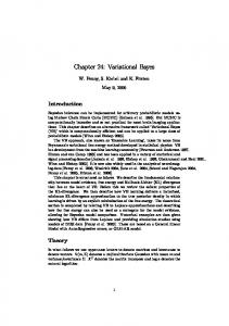
(a) Synthetic Image RMSE(10−2 ) SRE(dB )

Fig. 1.

Single Pixel BiICE 2.5013 2.5585 13.8106 13.7952 (b) Results

Joint Sparse 1.8621 13.8285

Synthetic Image and its results

To assess the accuracy of the proposed algorithm on the unmixing of homogeneous regions, a hyperspectral image is simulated according to the experimental settings of [4]. The simulated image was generated using a total of twelve endmember spectra, randomly selected from the USGS library, [6]. It comprises 150 × 150 pixels, with 25 homogeneous regions of size 20 × 20. Each pixel is mixed using up to five endmembers, with the homogeneous regions having no more endmembers than the identically generated background pixels, as shown in Fig. 1(a). The unmixing results are provided in Fig. 1(b). We observe that the proposed method outperforms its single pixel counterpart, both in terms of the RMSE and SRE. Thus, it becomes evident that the exploitation of the spatial information of homogeneous images can result in improved abundance estimation performance. contribution of the information provided by spatial correlation leads to better results compared to the case where no spatial information is considered. Next, the Cuprite data set, [2], [3], is used to illustrate the performance of the proposed scheme on real hyperspecral data. In this case, the Vertex Component Algorithm, [7], is first applied to the data set, in 3

Measure definitions can be found in [4].

May 12, 2014

DRAFT

7

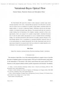
(a)Cuprite Image RE(10−3 ) SAM

Fig. 2.

Single Pixel BiICE 6.2712 5.9606 0.1633 0.1555 (b) Results

Joint Sparse 5.8313 0.1523

Cuprite image and its experimental results

order to extract N = 12 pure endmembers. Then, the proposed algorithm is applied to a subregion in the Cuprite data set, highlighted by the rectangular area in Fig. 2(a). The unmixing results are provided in Fig. 2(b). Again it is confirmed that the utilization of the existing spatial correlation in the selected area leads to higher estimation accuracy for the joint-sparse model, as compared to its single pixel variant, in terms of both the SAM and RE. VI. C ONCLUSIONS In this paper, a hierarchical Bayesian methodology for the semi-supervised unmixing problem, where the spatial correlation is taken into account, is introduced. As shown from the experimental results, the embodiment of the spatial correlation to our model leads to enhanced performance in terms of the accuracy of the estimations, when working on homogeneous regions of the images. R EFERENCES [1] W.K. Ma, J.M. Bioucas-Dias, Tsung-Han Chan, N. Gillis, P. Gader, A.J. Plaza, A. Ambikapathi, and Chong-Yung Chi, “A signal processing perspective on hyperspectral unmixing: Insights from remote sensing,” Signal Processing Magazine, IEEE, vol. 31, no. 1, pp. 67–81, Jan 2014. [2] K.E. Themelis, A.A. Rontogiannis, and K.D. Koutroumbas, “A novel hierarchical bayesian approach for sparse semisupervised hyperspectral unmixing,” Signal Processing, IEEE Transactions on, vol. 60, no. 2, pp. 585–599, Feb 2012.

May 12, 2014

DRAFT

8

[3] O. Eches, N. Dobigeon, and J-Y Tourneret, “Enhancing hyperspectral image unmixing with spatial correlations,” Geoscience and Remote Sensing, IEEE Transactions on, vol. 49, no. 11, pp. 4239–4247, Nov 2011. [4] Q. Qu, N.M. Nasrabadi, and T.D. Tran, “Abundance estimation for bilinear mixture models via joint sparse and low-rank representation,” Geoscience and Remote Sensing, IEEE Transactions on, vol. 52, no. 7, pp. 4404–4423, July 2014. [5] A.A. Rontogiannis, K.E. Themelis, and K.D. Koutroumbas, “A fast variational bayes algorithm for sparse semi-supervised unmixing of omega/mars express data,” in 5th Workshop on Hyperspectral Image and Signal Processing: Evolution in Remote Sensing (IEEE WHISPERS), Florida, June 2013. [6] R. N. Clark, G. A. Swayze, R. Wise, K. E. Livo, T. M. Hoefen, R. F. Kokaly, and S. J. Sutley, “USGS digital spectral library,” 2007, http://speclab.cr.usgs.gov/spectral.lib06/ds231/datatable.html. [7] J.M.P. Nascimento and J.M. Bioucas-Dias, “Vertex component analysis: a fast algorithm to unmix hyperspectral data,” Geoscience and Remote Sensing, IEEE Transactions on, vol. 43, no. 4, pp. 898–910, April 2005.

May 12, 2014

DRAFT