Author manuscript, published in "IEEE Transactions on Industrial Electronics (2010) 9" DOI : 10.1109/TIE.2010.2098358 1
IEEE TRANSACTIONS ON INDUSTRIAL ELECTRONICS
A Virtual Queuing based Algorithm for Delays Evaluation in Networked Control Systems
hal-00546532, version 1 - 14 Dec 2010
Boussad Addad, Saïd Amari and Jean-Jacques Lesage, Member, IEEE Abstract — In this paper, an approach to evaluate time performances of networked control systems (NCS) is presented. Switched-Ethernet with Client/Server protocol is considered for communication. As a result, the reactivity of these NCS is not only affected by the network delays but also by the field devices due delays. Obviously, all of them have to be taken into account to evaluate efficiently the NCS reactivity. So, by including some preliminary results, we propose an overall study in an effort to achieve this aim. First, we model the traffic of the NCS and provide formal proofs to characterize the scenarios leading to the worst delays. Subsequently, we develop a virtual queuing based algorithm (VQA) to search these scenarios and deduce the corresponding delays. Through a practical case study, it is shown how VQA fits experimental observations both quantitatively and qualitatively. Key words— Networked Control Systems, Client/Server Protocol, Switched Ethernet, Delays Evaluation, Virtual Queue
N
I. INTRODUCTION
OWADAYS, the industrial organizations are more and more sophisticated, consisting of many intelligent devices connected through communication networks. The widespread of networked control systems (NCS) was in essence motivated by reducing the volume of the wiring systems which are technically and economically a real issue. The bigger they are, the more difficult is their maintenance and the bigger is the bill of the consumed power (especially with embedded systems in vehicles). Beside NCS benefits however, some challenges have emerged too. The network due delays, which are often not constant or even random, affect dramatically the control loops. To deal with this tricky problem, many solutions have been developed according to the context and the application of the NCS. Approaching this problem can be achieved through two different ways. The control is synthesized by ignoring the delays while a network scheduling is performed so as to minimize the delays. Many communication protocols were developed for this purpose [1], [2], [3], [4]. The other approach is to firstly assess the network induced delays and subsequently look for an adequate control Manuscript received February 23, 2010; revised September 22, 2010; accepted November 18, 2010. B. Addad, S. Amari and J. J. Lesage are with the Automated Production Research Laboratory LURPA, ENS-Cachan, 94235 Cachan Cedex, France (email:
[email protected];
[email protected];
[email protected]).
strategy to compensate the negative effect of the delays. During the last years, this topic has been actively investigated and many advanced control strategies have been proposed [5], [6], [7], [8]. In the majority of these studies however, only the network due delays have been considered [9], [10], [11] i.e. the network delays affecting a packet when traveling from a sensor to a controller and from a controller to an actuator. With Client/Server protocols like Modbus TCP [12], one of the most widespread protocols in industry, this assumption is actually no longer viable. Indeed, two different issues are to be investigated at the same time: the network delays on one hand and the field devices due delays on the other hand. Moreover, the latter delays are often by far larger than the network delays. As a matter of fact, no complete investigation has been carried out so as to evaluate the real time capabilities of such NCS. The rare related works are often simulation of some scenarios [13], [14], [15] without being exhaustive. In doing so, the critical cases that correspond to the worst delays are not guaranteed to be found. When it is the case using exhaustive methods like model-checking [16], [17], only relatively simple architectures are targeted because of the classical state explosion problem of this method. Also, a trivial method that consists of adding up the worst local delays is possible but it is so pessimistic (50% overestimation) that it is not practically viable [18]. So, the aim of this paper is to avoid the state explosion while considering enough large NCS. Also, a formal proof of an accurate and exhaustive exploration is provided while taking into account both the network and the field devices delays. The remainder of this paper is organized as follows: an overview of Client/Server NCS and the context of the study are discussed in Section II. Then in Section III, an analysis about the traffics interference is addressed and the worst scenarios are identified. Thereafter, a virtual queuing based algorithm (VQA), to calculate the delays corresponding to these scenarios, is proposed in Section IV. Afterwards in Section V, a practical case study is considered for validation. Finally, some concluding remarks are given in Section VI. II. BACKGROUND As aforementioned, we consider an NCS that works according to Client/Server protocol. It is constituted of PLCs (programmable logic controllers), remote input output modules (RIOMs), PCs to perform high level functions and finally a switched Ethernet network for communication (Fig. 1). The PLC comprises two modules, the CPU (central processing unit) that executes the user program to perform the
IEEE TRANSACTIONS ON INDUSTRIAL ELECTRONICS
2
control signal and an Ethernet board for communication. To explain the functioning of such NCS, an example of automated plant is depicted in Fig. 1. It consists of filling a tank and maintaining the level of water around a height hr by operating a pump as long this level is not reached. This is achieved as follows: PLC2 (client) sends periodically requests to RIOMs R13 and R16 (servers). By using the information got from a level detector (connected to R13), a decision is performed by PLC2 and sent to the pump trigger (R16).
- Load: delays due to waiting for the shared resources availability e.g. a request arriving to a RIOM is processed only after all the waiting requests are (hatching in d1 ).
RTT
NFD R12 detector
source
1
RIOMs Net
2
ETHb
3
CPU
4
R15 R16
hal-00546532, version 1 - 14 Dec 2010
PLC1
R17
Network PLC3
destination
d1
d7
d3 TCPU
8 7
d6
d2
6
d5
5
d4
NFD
RTT
hr
R14
Load
Dr
Plant
R13
PLC2
Asynchronism
Intrinsic
TETHb
tank filling pump
R18 R19 RIOMs
Fig. 1. Example of Client/Server NCS.
Actually, the aim is to maintain the level around hr but above all to surely avoid overflows while filling the tank. This depends on the maximal bound of the response time of the NCS and the tank itself. The response time noted Dr is defined as the delay between the date of reaching level hr and the date of stopping the pump. Thus, the maximal bound of Dr must be smaller than the necessary time to fill the volume of the tank from the detector level to the top edge (hatched in Fig. 1). Hence, we notice the importance of this delay and its role in the NCS safety. Also, its impact on the stability and the quality of control was shown in [18]. The evaluation of maximal bound of the response time is therefore of top priority. This is the main aim of our study. As a matter of fact, the evaluation of the response time of such a system is tricky. This is mainly due to the non synchronization of the components and the absence of a global scheduling of the shared resources in the NCS. In Fig. 2, the response time can be seen as the sum of three types of delays at every stage of the NCS: Dr = ∑ d k (1) - Intrinsic delays: they are the inevitable delays due to the resources capacities (e.g. the delay to execute the user program and perform the control signal ( d 4 )). - Non synchronization: they are delays due to the non synchronization of the different components. For example, a new value in the detector output is taken into account only after the arrival of a request from PLC2 (black part of d1 ).
Fig. 2. Response time decomposition into three types of delays; intrinsic delays, delays due to non synchronization and finally delays due to load (waiting for resources availability).
According to the results exposed in [19], Dr depends on two major time features, the round trip time (RTT) and the network forwarding delay (NFD). The obtained formula of the maximal response time was given as: DMAX ≈ (q + 1) ⋅ TETHb + Δ NFD + d 7 (2) where q is the minimal integer that verifies inequality: q > ( RTT + TCPU + d 4 ) / TETHb . All the parameters in (2) are
depicted in Fig. 2; The RTT is the delay between the date of sending a request from PLC2 and the date of arrival of the returned answer from R13 (Fig. 1-2). The NFD is the necessary delay, to forward across the network, the control signal issued from PLC2 to the destination R16 (Fig. 1-2). Thus, Δ NFD is the jitter (difference between the maximal and the minimal value) of the delay NFD. Timing features TETHb , TCPU , d 4 , and d7 are respectively the period of the Ethernet
board, the period of the CPU of PLC2, the necessary time to execute the user program in the CPU, and finally the necessary time to process the request in the destination RIOM R16. Actually, formula (2) gives an upper bound of the response time but the exact value of the maximal response time is a bit more complicated [19]. Obviously, one can tackle the problem differently by considering an upper bound as the addition of the theoretical maximum values of the local delays d k : DMAX = ∑ max {d k }
(3)
Unfortunately, in such complex systems these different delays are dependent of each other. When the response time is maximal, it does not mean that all these local delays reach their maximal values at the same time. An example in [18] showed that using equation (3) led to an overestimation of the real maximum bound with about 50%. As a result of this very
IEEE TRANSACTIONS ON INDUSTRIAL ELECTRONICS pessimistic evaluation, the quality of control in the NCS was degraded to guarantee stability [18]. Using equation (2) however, led to a satisfactory result with an overestimation of only 1%, resulting in a much better quality of control. On top of that, a thorough analysis in [19] showed that the maximum bound DMAX is reached when both the NFD and the RTT are maximal. Hence, we propose an approach to assess the maximal bounds of the RTT and the NFD so as to eventually use them in (2) to evaluate efficiently DMAX .
hal-00546532, version 1 - 14 Dec 2010
With Client/Server paradigm, the RIOMs are scanned periodically by the controllers. For instance, in Fig. 1-3, PLC2 sends five requests f12 , f 22 , f32 , f 42 and f52 to respectively RIOMs R12 , R13 , R14 , R15 and R16 . To assess the RTT relative to the control loop of Fig. 1, we have to find the delay that the frame f 22 (hatched in Fig. 3) experiences when crossing the network. Since the FIFO (First in First out) scheduling is considered in the switch of the network, when the frame f 22 enters the switch at the date denoted by t*, it experiences a delay that depends solely on the set of frames that entered the switch before it. Let us denote this set by E as in Fig. 3.
(a)
f 21
f 31
f11
t − δ1 f1 2 *
f 52 f 42
f 32
f 22
PLC1
E t −γ *
t
f
3 4
f
3 3
f
3 2
f
3 1
PLC 2
PLC 3
t − δ3 *
(b )
f 41 f 52 f 42
f 31 f 22
f 32
t t
f
3 4
f
f 21
δ1
f11
PLC1
E
f1 2
PLC 2
* 3 3
f
3 2
f
δ3
3 1
PLC 3
t − γ + δ1 *
A. Lemma Let f 22 be the frame under consideration and its arrival date into the switch be t*. Let E be the set of frames arriving before f 22 and the frames from the parallel controllers entering immediately before f 22 be f31 and f33 (grayed in Fig. 3). Thus, we can formulate the following lemma: If the set E corresponds to the worst scenario, than the worst delay is experienced if and only if the frames f31 and f33 entered the switch immediately before f 22 . In other
III. TRAFFIC MODELING AND ANALYSIS
f 41
3
Fig. 3. Analysis of the frames interference, (a) before shifting frames, (b) after shifting frames.
This set corresponds also to the quantity of work (backlog) waiting to be processed at date t*. Let us denote this backlog by w(t*). The challenge is then to find the scenario (set E) that corresponds to the worst delay that frame f 22 undergoes. The next lemma does not give precisely the worst scenario but provides an important propriety to identify it.
words, the arrival date of f31 and f33 is t * − ε where ε > 0 tends to zero. Proof (by contradiction): Suppose that the worst case delay noted Δ is reached when the frames f31 and f33 enter at date t * − δ1 and t * − δ 3 respectively as in Fig. 3(a) and the backlog at t* is w(t*). Let us now shift the groups of requests from PLC1 and PLC3 with the lags δ1 and δ 3 (this is possible since the PLCs generate their requests independently from each other) while keeping the frames f31 and f33 enter the switch before f 22 as in Fig. 3(b). Thus, the set E of frames preceding f 22 remains the same but the quantity of work is no longer w(t*) but w'(t*) and the corresponding delay is Δ ' . So, the frames from PLC1 enter δ1 later than they do in the first case (case before shift) and the frames from PLC3 enter δ 3 later. Since the set E remains the same, then the backlog w'(t*) is necessarily greater than w(t*) and therefore the delay Δ ' is greater than Δ . Indeed, when the same set E begins to be processed at a later date, the processing is finished later too. Obviously, stating that Δ ' is greater than Δ is absurd since from the beginning Δ is supposed to be the worst delay. ■ The previous lemma provides us with important information to identify the worst case scenario but the set E that corresponds to it is still unknown. All we know is that the worst delay is reached when f 22 enters a bit after two frames ( fi1 , f j3 ) from the parallel controllers PLC1 and PLC3. So,
we can check every combination ( fi1 , f j3 ) for 1 ≤ i ≤ 4 and
1 ≤ j ≤ 4 and then simulate the system behaviour according to the lemma. Actually, such a method would not be viable in general since it is not easy to identify discrete dates in systems that display uncertainties and complex configurations. So, instead of looking for these discrete dates, we rather search for the set E. As we saw before however, the knowledge of this set is not sufficient since case (a) and case (b) correspond to the same set E but not the same delay. Fortunately, the next theorem will prove that if the set E remains the same but we know how much the parallel frames are shifted with (at least the maximum shift), then the discrepancy of the corresponding delay from the worst one is known as well.
IEEE TRANSACTIONS ON INDUSTRIAL ELECTRONICS B. Theorem Let the start-sending dates from PLC1 and PLC3 be (t * − τ1 ) and (t * − τ 3 ) respectively. In other words, (t * − τ1 ) is the arrival date of f11 and (t * − τ 3 ) is the arrival date of f13 . Looking for the worst scenario is obviously equivalent to looking for the corresponding lags τ1 and τ 3 . If a step δ e , smaller than the minimal inter-arrival time, is used to vary the lags τ1 and τ 3 in a combinatorial scheme, then we have the following: i) An exhaustive exploration is achieved and the set E that corresponds to the worst case is surely swept. ii) The accuracy of the assessed worst delay Δ is worth δ e . In other words (Δ worst − Δ ) ≤ δ e . Proof: i) the first result is straightforward. Indeed, the date * t varies with a step δ e smaller than any inter-arrival period
hal-00546532, version 1 - 14 Dec 2010
of two consecutive frames from PLC1 ( fi1 and fi1+1 ). As a consequence, when varying the lags, t * is surely between the dates of arrival of two consecutive frames fi1 and fi1+1 . In the case of Fig. 3, when τ1 varies with a step δ e , we are sure to obtain t * between the arrival dates of f31 and f 41 . Thus, the subset of E from PLC1 is found. The subset from PLC3 is obtained in exactly the same way. ii) The set E is found but we obtain a configuration as on Fig. 3(a), not the worst case of Fig. 3(b). Indeed, we obtain arrival dates of f31 and f33 to be t * − δ1 and t * − δ 3 where δ1 ≤ δ e and δ 3 ≤ δ e . The worst drift from case (b) is when
δ1 = δ 3 = δ e . This means that the frames from PLC1 and PLC3 enter the switch δ e units of time earlier. Consequently,
4 an exhaustive one as aforementioned in the introduction. So, the bounds of the delays are not guaranteed to be found. Basically, this was the main incentive behind the introduction of VQA (virtual queuing based algorithm) though it can be used in other contexts other than Client/Server NCS [20]. IV. VIRTUAL QUEUING BASED ALGORITHM The algorithm we are going to present is based on some concepts we need to explain: Virtual Queuing (VQ) and Free Access Date (FAD). A. Definitions 1) Virtual queuing Virtual FIFO queue (VFQ): a virtual queue (VQ) is a concept we associate to a real queue (input port in a switch). At a given time, a VQ not only contains all the frames that have been already received by the real one but also all the frames that will be received in the future, provided that the dates of their arrivals be known. More formally, it is a set < f , θ > where f = { ASCR , ADST , L} is a frame of length L , issued from a device (e.g. PLC) with address ASCR and going to the destination address ADST . Component θ is the date of arrival of the frame to the switch. At given date t , some of the waiting frames have already quitted the VQ (black on Fig. 4) and others are still waiting (gray on Fig. 4). So, to know at each time the frame that is waiting to be forwarded first, we associate to each VQ a counter as in Fig. 4. Since there are multiple ports in a switch, we associate to each port a VQ. So, we note < f qp , θ qp > the qth frame of the VQ relative to the p th port. Its counter is noted n p . Still waiting
Already forwarded
the frame f 22 will be forwarded at best δ e earlier. So, the frame f 22 experiences a delay Δ with Δ ≥ Δ worst − δ e . This can be written equivalently as: (Δ worst − Δ ) ≤ δ e . ■ Remarks III.1: - Since an overestimation of the worst delay is sought, it is enough to add δ e to the assessed delay to obtain Δ + δ e ≥ Δ worst (consequence of result (ii)).
- Once the set E corresponding to the worst case is found, we can tighten the step δ e so as to improve the precision of the worst delay assessment (see the case study of Section V). The issue now is to determine how the system behaves for a given set of lags τ i . Then, by performing an exhaustive exploration, according to the previous theorem, the maximal bound of a delay is deduced. To the best of our knowledge, no suitable discrete event simulator is available to achieve this purpose. The features of Client/Server protocol along with the presence of the RIOMs are the main obstacles to that. In an effort to solve this problem, an investigation has already been carried out in [15]. Unfortunately, the proposed method is not
( f 75 , θ 75 )
n5 = 3
Fig. 4. The virtual queue n°5 (input port 5).
The VQ is said to be FIFO or VFQ if θ(pq +1) ≥ θ qp , ∀p, q ≥ 1 i.e. the frames are ordered according to their arrivals into the real queue. The first arrived is the first to be forwarded. When a frame is forwarded, the counter is increased so as to point the potential following frame to depart in the future. That way, we know all the pending frames in all the VFQs at any time. 2) Free access date As aforementioned, no global scheduling of the resources is available in the NCS. So, considerable and variable delays due to waiting for access to the shared resources are experienced. The date at which access is possible to a shared resource is called “Free Access Date” (FAD). Thus, we associate a FAD to each shared resource of the NCS. Naturally, the shared resources depend on the models used in the study. In our case (Fig. 5), we use the same switch model considered in [2]. It
IEEE TRANSACTIONS ON INDUSTRIAL ELECTRONICS
5
Start (l = 0) l = l +1
Generate the start-sending dates Deduce the arrival dates and feed the VFBs
Find the frame to forward; the k th VFQ is selected and its leading frame f = { ASCR , ADST , L} is to be forwarded to the s th output port
u ϑ1 = θ (kn k + 1) + L / C ink , ϑ 2 = m ax(ϑ1 , Fsw )
ϑ 3 = ϑ 2 + L / C , ϑ 4 = m ax(ϑ 3 , F Hs O L ) s ϑ 5 = ϑ 4 + L / C out ,
s F Hs O L = ϑ 5 + L IF G / C out
PLC
hal-00546532, version 1 - 14 Dec 2010
Switch The receiver is a: Feed the r th VFQ
RIOM
Other
No
ASRC = κ Sens & ADST = κ PLC
s s s ϑ6 = max(ϑ5 , FRIOM ), FRIOM = ϑ6 + T RIOM
Yes
l s DRTT = FETHb − θηκ PLC sen
Feed the s
th
VFB Yes
No
Any waiting frames?
ASRC = κ PLC & ADST = κ act
Search finished?
Yes l s D NFD = FRIOM − θηκ PLC act
No
No
Yes MAX l DRTT = max( DRTT ), l
MAX l D NFD = max( D NFD ) l
End Fig. 7. Flowchart of VQA.
involves a central dispatcher that forwards the frames according to FIFO scheduling, at a speed (bits/s) noted C . In considering a "store & forward" switch, a frame is completely received before being forwarded by the dispatcher to the appropriate egress port. The data are exchanged with the end stations (PLC or RIOMs) at a bitrate (bits/s) corresponding to k physical links capacity, noted Cink or Cout for port k (Fig. 5). When a RIOM receives a request, at the bitrate of the switch k port Cout , it buffers it in a FIFO queue until all the waiting frames are processed. Then, it processes it during a time
s TRIOM before to return an answer at a bitrate Cins .
According to the models of Fig. 5, we can easily identify the following shared resources and their FAD: u - Fsw : FAD to the dispatcher of the switch number u (the dispatcher can forward only one frame at a time). s - FHOL : FAD to the HOL (head-of-line) of the output port s (leaving an output port is possible only after all the frames in the head of the queue are retransmitted out of the switch). s - FRIOM : FAD to the processor of the RIOM connected to the
IEEE TRANSACTIONS ON INDUSTRIAL ELECTRONICS
6
port s (a RIOM can process only one request at a time). The main notions we handle being defined, we will explain step by step the algorithm VQA.
- PLC2 sends a request periodically with a period T2 to module R11. We can note from Fig. 6(a) that all the ports of the switches are numbered differently (Sw1: 1, 2, 3; Sw2: 4, 5, 6, 7). So, we talk about the k th port of the system ascribed the
HOL
Switch
1 Cin
1 C out
C 2 C out
C in2 Dispatcher
CinN
N C out
Egress ports
Ingress ports
FIFO
FIFO
s Delay TRIOM
hal-00546532, version 1 - 14 Dec 2010
Fig. 5. Devices modeling using queues and shared resources
B. Virtual queuing based algorithm (VQA) The flowchart drawn in Fig.7 displays all the steps to achieve delays evaluation using VQA. The variables ϑi in the flowchart are only introduced for a better structuring of the algorithm and improving its clarity. The idea behind VQA is to look at every step, among all the competing VFQs, which one will have access to the shared resources. When a VFQ is selected, its leading frame is forwarded until it reaches another VFQ or simply quit the system. Meanwhile, the FADs are updated and the contents of the competing VFQs as well. The mechanism is repeated until all the VFQs are empty. To explain as clearly as possible the method, a relatively simple system shown in Fig. 6(a) is used. The corresponding scanning mechanism is in Fig. 6(b): (a) Sw2
Sw1
1 PLC1
3
4
R11
5 sensor
6 2
R12
7
actuator R13
Reference time
Burst of frames
LIFG
T1
PLC1
θ11 PLC2
f11
(b)
θ 21 τ
T2
- κ sen is the address of the sensor. In Fig. 6(a), the sensor is - κ act is the address of the actuator. In Fig. 6(a), the actuator
2 C out
Processing
PLC2
In Fig. 6(a), it is PLC1, so κ PLC = 2 . connected to R12 and therefore κ sen = 6 .
RIOM
Cin2
k th virtual FIFO queue. In such a way, we can use as an address of each station only the number of the port that connects it to the network. Thus we adopt the following notations: - κ PLC is the address of the controller of the loop in question.
f12
to R12 η sen = 1
f 21 to R13 η act = 2
is connected to R13 and therefore κ act = 7 . Since the controller may send a burst of several requests to the RIOMs (e.g. PLC1 in Fig. 6(b)), we have to identify the frames that are involved in the loop in question; the request sent to the sensor and the one sent to the actuator. Therefore, we identify them by their rank in the burst: - η sen is the rank of the frame sent to the sensor ( η sen = 1 in the example of Fig. 6). - ηact is the rank of the frame sent to the actuator ( ηact = 2 in the example of Fig. 6). The notations being defined, we can explain VQA: - Step0 (initialization of VQA): First of all, we generate the dates of start sending the frames from the PLCs; θ11 and θ12 . We put the date of start sending of one of them as a reference and the others are generated with lags from it. In Fig. 6(b), the reference is PLC1 and the start-sending date of PLC2 is generated with a lag τ from it. The start-sending dates of the leading requests in each burst being known, the arrival dates to the switch Sw1 of the following frames are deduced. In the example, θ 21 is deduced using the length of frame f 21 , the inter-frame gap LIFG , and the bitrate of port 1. So, we can already feed the VFQs number 1 and 2 (of the ports linking the PLCs to Sw1). The counters of the VFQs are all set to zero since no frame has already been forwarded ( nk = 0, ∀k ). - Step1: among all the non empty VFQs (#1 and #2 at this step), we select the one whose the HOL (leading frame that waits to be forwarded first) has the minimal date. If it is the k th VFQ of the switch number u , then it must verify:
θ (knk +1) = min(θ (pn p +1) ) . The frame to be forwarded is supposed p
θ12
to R11
Fig. 6. (a) Example of NCS, (b) Scanning mechanism.
- PLC1 sends a burst of two requests periodically with a period T1 to modules R12 and R13.
to be f = { ASCR , ADST , L} and the egress port that will receive it is the s th port (to be determined using a look-up table). If we look at the scenario drawn in Fig. 6(b), the selected frame
{
}
is f11 since θ11 = min θ11 , θ 21 ,θ12 . The egress port is s = 3 .
IEEE TRANSACTIONS ON INDUSTRIAL ELECTRONICS
7
- Step2: the frame is selected but the forwarding is possible u ) with ϑ1 = θ (knk +1) + L / Cink i.e. only at date ϑ2 = max(ϑ1 , Fsw
problem by constraining the data emission; a sensor does send a message only if its state changes. Fortunately, the concepts of VFQ and FAD are enough generic to be extended easily to these protocols without changing the core of VQA. This can be achieved quite straightforwardly by inverting the roles of the controllers and the sensors. A sensor can be considered as client that sends requests whereas a controller as a server that returns answers. The necessary time to a request to be processed by a controller is the time to execute the user program, noted d 4 previously in Section II. Nevertheless, in considering such protocols, one has to take care about the information broadcast by a sensor. In event there are many consumers of this information, multicast has to be taken into account in the models of the NCS components and VQA has to be adapted accordingly.
the frame is completely received (store & forward switch) and the dispatcher u is free. - Step3: the frame is received completely at the egress line at date ϑ3 = ϑ2 + L / C but once again, the frame can exit the switch only after the HOL of egress port s is free i.e. at date s ϑ4 = max(ϑ3 , FHOL ) . Hence, the frame exits completely the
hal-00546532, version 1 - 14 Dec 2010
s switch at date ϑ5 = ϑ4 + L / Cout . The FAD of the HOL of egress port s is updated using this date and the inter frame s s = ϑ5 + LIFG / Cout . gap LIFG : FHOL - Step4: at this point, four cases can be analyzed depending on the type of the receiver of the previous frame; a switch, a RIOM, a PLC or another station (e.g. a PC that does not return answers). a) Switch (e.g. a frame that exits from port 3 to enter port 4): if the port of this receiving switch is ascribed the number r , then the r th VFQ is fed with the previous frame. Go to Step1. b) RIOM: in this case, the frame will wait in the FIFO buffer of requests until the access is free to the RIOM s ) . Then, it is processed and a processor: ϑ6 = max(ϑ5 , FRIOM response is returned. This answer is received at the input port s (which was an output port previously). So, the VFQ s is fed with the response frame and the FAD of the RIOM is updated. Hence, we make a test if this RIOM is the control signal destination R13 and the source address of the frame is PLC2. If it s the case, the NFD can be calculated. Go to Step1. c) PLC: Here also, we make a test if this PLC is the sender of the control signal (PLC2) and the RIOM that returned the answer is R12. If it is the case, the RTT can be calculated. Go to step 4(d). d) A station without answer (including PLCs): in this case, we only check if there are waiting frames in the different VFQs of the NCS. If it is the case, then go to Step1, else the algorithm is terminated. The previous algorithm is run for a particular set of startsending dates. The algorithm is repeated as many times as necessary according to the theorem of section II so as to find the critical scenario. This is represented using the exploration loop (index l) on the flowchart which finishes by the calculus of the maxima of the delays RTT and NFD: MAX l MAX l DRTT = max( DRTT ) and DNFD = max( DNFD ).
l
l
Remarks IV.1: While Client/Server protocol (e.g. Modbus TCP [12]) displays many advantages, that justify its widespread in industry automation, the continuous periodic scanning of the remote modules would be a disadvantage in some cases. Indeed, when a client asks continuously for a sensor data while this latter do not change during many cycles, it results unnecessarily in an overcrowded network. Other protocols like Producer/Consumer (e.g. ProfiNet [3]) bypass this
V. CASE STUDY: APPLICATION AND VALIDATION The system is represented in Fig. 8 and includes two parts: PART I and PART II. PART I works as follows: Three controllers, PLC1, PLC2, and PLC3 scan respectively the ordered sets of RIOMs: {R12 , R13 , R14 } , {R14 , R15 , R16 } and {R16 , R17 } . Minimal length Ethernet frames of 64bytes are used for scanning the RIOMs in a first case and 89bytes frames in a second case. The two cases are considered so as to figure out the influence of the frames length on the delays. PART I is the automation part as the one we used for explanation in Section II but as stated previously, the studied system presents the advantage of easiness of high level functions integration (since standard Ethernet is used for communication). So, a second part PART II with such a role is connected to this sub-network; PC1 sends long frames of 1000Bytes length to the stations PC3 and PC4. PC2 has the role of a supervisor of PART I. It scans all the RIOMs every 300ms so as to check the good functioning of the NCS. All the links of the switches are configured to work at a full duplex s in mode with a speed of 10Mbps. The processing times TRIOM the different RIOMs are very slightly variable in practice. Indeed, experimental measures performed on a RIOM [21], led to a maximal value of 0.5471ms and a minimal one of 0.5428ms i.e. less than 0.8% jitter. So, rounded up values are TABLE I REQUESTS PROCESSING DURATIONS IN THE RIOMS ( in
ms )
R12
R13
R14
R15
R16
R17
0.50
0.60
0.70
0.55
0.60
0.50
used in our study as given in Table I. Now, the aim is to evaluate upper bounds of the delays RTT and NFD relative to the control loop represented in Fig. 8; PLC2 is the controller, R14 the source of information (sensor) and R16 the destination of the control signal (actuator). The evaluation was performed with different conditions of load so as to analyze the influence of the parallel traffic on this loop. Many cases were considered by removing one or more
IEEE TRANSACTIONS ON INDUSTRIAL ELECTRONICS stations from the system. In each case, the removed components are mentioned in Table II. Case 0 where no load is present (all the flows affecting the loop are removed) was the reference of our analysis. Hence, VQA was applied by taking into consideration the previous theorem conditions. With Ethernet, we can easily calculate the minimal interarrival time as: δ = (64 + preamble + LIFG ) /(10Mbps) = 67.2μ s . So, the exploration step δ e must be smaller than this value. A progressive narrowing of the step δ e is performed with the condition checked: δ e = 50 μ s then 10μ s and finally 1μ s . The final results are reported in Table II.
P A R T
Sw1 PC1
PC3
hal-00546532, version 1 - 14 Dec 2010
II PC2 PLC1
PC4 R12
Sw2
R13 R14
PLC2 RTT R15 Sw3
NFD
P A Sensor R Actuator T
R16
I R17
PLC3
Fig. 8. Client/server NCS: Case study.
As expected, whatever is the length of the frames, the delays RTT and NFD had their smallest values in Case 0. Depending on the removed traffic, either RTT or NFD changed while the following observations were noticed: 1) RTT: as we can notice, PLC3 had no influence on RTT since no effect was observed when it was added from Case 0 to Case 1. This is simply due to the fact that no intersection exists between the RTT path and PLC3 requests path. When PLC1 or PC2 was added however (Case 2 and Case 3), an additional delay of about 0.7ms was noticed. When they were present at the same time, twice this value was added (Case 4) and a variation of the RTT of about 130% from Case 0 to Case 4 was observed. The little difference between Case 2 and Case 3 is due to the effect of sharing the resource Sw2. As a matter of fact, the value of 0.7ms is the necessary delay to process a request in R14 (see Table I). So, the more it is shared by clients the more the request from PLC2 suffers when waiting for the module R14 processor availability. 2) NFD: almost the same phenomenon was observed with NFD. Indeed, when a client of the module R16 was added (Case 1 and Case 2), an extra delay of about 0.6ms was
8 TABLE II RESULTS OF EVALUATION USING VQA Case 0
Case 1
Case 2
Case 3
PC2, PLC1, PLC3
PC2, PLC1
PLC1
PC2
64B
1.10
1.10
1.86
1.80
2.56
89B
1.23
1.23
1.99
1.90
2.72
64B
0.91
1.51
1.51
2.11
2.11
89B
0.96
1.53
1.53
2.19
2.19
Removed components RTT (ms )
NFD (ms )
Case 4
noticed and twice this value when two clients were present (Case 3 and Case 4). It followed a variation of about 128% from Case 0 to Case 4. The time to process a request in R16 is also equal to 0.6ms. 3) The network delay (experienced exclusively in the switches): when all the flows were present and therefore the network maximally crowded (Case 4), the pure network delay-to-RTT ratio was less than 20%. The same proportion can be estimated with respect to NFD. Hence, we get to the same conclusion stated previously in Section II; the sole pure network delay is not enough to carry out an efficient evaluation of this NCS time performances. The whole architecture is to be considered in the study. 4) The frames length: the effect of changing the length of the frames was maximal in Case 0 with a ratio of about 5% for NFD and 10% for RTT. Hence, we can conclude that the impact of the frames length and the parallel traffic (affecting the pure network delays) are much smaller than the effect of sharing the RIOMs. 5) The response time: by setting the scanning period of PLC2 to 10 ms and the CPU period to 5 ms, the use of formula (2) led to an upper bound of the response time of about 22.6ms in Case 0 and 23.7 ms in Case 4 (both cases using 89bytes frames). This means a tight overestimation of the experimental value (22.3ms [22]) with only 1.5%. So, both overestimation and accuracy were achieved at the same time. We can also point out that the effect, on the response time, of sharing the RIOMs was of about 6% (calculated as: (2.190.96)/22.3). So, all the conclusions of this study fit the experimental ones of [22] where it was stated that the effect of the network components and the frames length are not striking whereas sharing the RIOMs causes less than 10% effect.
VI. CONCLUSION In this paper, we proposed a method to assess switchedpackets delivery delays in the context of Client/Server networked control systems. A virtual queuing based
IEEE TRANSACTIONS ON INDUSTRIAL ELECTRONICS
9
algorithm (VQA), taking into account both the field devices and the switches, was developed for this purpose. Moreover, a formal proof was provided about the capacity of VQA to achieve exhaustive exploration and sweep the worst delays. Thereafter, it was showed that VQA fits different experimental observations and provides satisfactory results. Thus, instead of making thousands of onerous experimental measures, VQA is a satisfactory alternative with efficient delays evaluation.
[19] B. Addad, S. Amari, and J. J Lesage, “Analytic calculus of response time in networked automation systems”, IEEE Trans. on Automation Science and Engineering, 7(4), pp. 858-869, 2010. [20] B. Addad, S. Amari and J-J. Lesage, “Evaluation de délais dans les systèmes de communication temps réel en utilisant des files d’attente virtuelles”, MSR - Journal Europeen des Systemes Automatisé (JESA), 43(7-9), pp. 985-1000, 2009. [21] G. Marsal, Evaluation of time performances of Ethernet based automation systems by simulation of high level Petri nets. PhD thesis, ENS Cachan (France) and Kaiserslautern University (Germany), 2006. [22] B. Denis, S. Ruel, J.-M. Faure, and G. Marsal, “Measuring the impact of vertical integration on response times in Ethernet fieldbuses”, In Proc. of ETFA07, Patras, Greece, pp. 532-539, 2007.
REFERENCES [1] [2] [3]
hal-00546532, version 1 - 14 Dec 2010
[4] [5]
[6] [7]
[8]
[9] [10]
[11] [12] [13]
[14] [15] [16]
[17] [18]
P. Neumann, “Communication in industrial automation: what is going on?”, Control Engineering Practice, 15(11), pp. 1332-1347, 2007. J. Jasperneite, J. Imtiaz, M. Schumacher, and K. Weber, “A Proposal for a Generic Real-Time Ethernet Systems”, IEEE Trans. on Industrial Informatics, 5(2), pp. 75-85, 2009. J. Kjellson, A. E. Vallestad, R. Steigmann, and D. Dzung, “Integration of a Wireless I/O Interface for Frofibus and Profinet for Factory Automation”, IEEE Trans. on Industrial Electronics, 56(10), pp. 42794287, 2009. L. Seno, S. Vitturi, and C. Zunino, “Analysis of Ethernet Powerlink Wireless Extensions Based on the IEEE 802.11 WLAN”, IEEE Trans. on Industrial Informatics, 5(2), pp. 86-98, 2009. K. Natori and K. Ohnishi, “A design Method of communication Disturbance Observer for Time-Delay Compensation, Taking the Dynamic Property of Network Disturbance Into Account”, IEEE Trans. on Industrial Electronics, 55(5), pp. 2152-2168, 2008. X. Tian, X. Wang, and Y. Cheng, “Self-tuning fuzzy controller for networked control system”, International Journal of Computer Science and Networks Security, 7(1), pp. 97-102, 2007. G. P. Liu, Y. Xia, J. Chen, D. Rees, and W. Hu, “Networked Predictive Control of Systems with Random Network Delays in Both Forward and Feedback channels”, IEEE Trans. on Industrial Electronics, 54(3), pp. 1282-1297, 2007. K. Natori, T. Tsuji, K. Ohnishi, A. Hace, and K. Jezernik, “Time Delay Compensation by Communication Disturbance Observer for Bilateral teleoperation Under Time-Varying delay”, IEEE Trans. on Industrial Electronics, 57(3), pp. 1050-1062, 2010. R. L. Cruz, “A calculus for network delay, Part I: network in isolation”, IEEE Trans. Information Theory, 37(1), pp. 114-131, 1991. J. P. Georges, E. Rondeau, and T. Divoux, “Confronting the performances of switched Ethernet network with industrial constraints by using Network Calculus”, Communication Systems, 18(9), pp. 877903, 2005. K. C. Lee, S. Lee, and M. H. Lee, “Worst case communication delay of real time industrial switched Ethernet with multiple levels”, IEEE Trans. on Industrial Electronics, 53(5), pp. 1669-1676, 2006. MODBUS Messaging on TCP/IP Implementation Guide V1.0b, (October 2006), [Online]. Available: www.modbus-ida.org/specs H. D. Witsch, B. Vogel-Heuser, J.-M Faure, and G. Poulard-Marsal, “Performance analysis of industrial Ethernet networks by means of timed model-checking”, In Proc. of 12th IFAC INCOM, St-Etienne, France, pp. 101–106, 2006. D.A. Zaitsev, “Switched LAN simulation by colored Petri nets”, Mathematics and Computers in Simulation, 65(3), pp. 245–249, 2004. G. Marsal, B. Denis, J.-M. Faure, and G. Frey, “Evaluation of response time in Ethernet-based automation systems”, In Proc. of ETFA06, Prague, Czech Republic, pp. 380-387, 2006. J. Greifeneder and G. Frey “Probabilistic Timed Automata for Modeling Networked Automation Systems”, In Proc. of the 1st IFAC Workshop on Dependable Control of Discrete Systems DCDS, pp. 143-148, Cachan, France, 2007. S. Ruel, O. DE Smet, J.-M. Faure, “Finding the bounds of response time of networked automation systems by iterative proofs”, In Proc. of 13th IFAC INCOM, Moscow, Russia, pp. 1365-1370, 2009. B. Addad and S. Amari, “delay evaluation and compensation in Ethernet networked control systems”, in Proc. 16th Int. Conf. RTNS Real Time and Network Systems, Rennes, France, pp. 139-148, 2008.
Boussad Addad received the Engineer degree in control systems from the National Polytechnic School of Algiers, Algiers, Algeria, in 2007, and the M.S degree in automated systems engineering from the Ecole Normale Supérieure de Cachan, Cachan, France, in 2008, and is currently working toward the Ph.D. degree at the Ecole Normale Supérieure de Cachan, Cachan. His research interests include modeling and analysis of discrete event systems along with time performance evaluation of networked automation systems.
Saïd Amari received the Ph.D. degree from the Institute of Research in Communications and Cybernetic of Nantes, Nantes, France, in 2005. He is currently an Associate Professor at the University of Paris XIII. He carries out research at the Automated Production Research Laboratory from the École Normale Supérieure de Cachan. His main research interests are performance evaluation and control of Discrete Event Systems with Petri nets and Dioid algebra.
Jean-Jacques Lesage (M’07) received the Ph.D. degree in 1989, and the “Habilitation à Diriger des Recherches” in 1994 from the University Nancy 1 Henri Poincaré, Nancy, France. He is currently a Professor of Automatic Control at the École Normale Supérieure de Cachan, Cachan, France. His research topics are formal methods and models of Discrete Event Systems (DES), both for modeling synthesis and analysis. The common objective of his works is to increase the dependability of the DES control.